3.4. Exercises#
Exercise 3.13
Last week you used the following equations to model the dynamics of the Belousov–Zhabotinsky reaction where \(X_i\) and \(Y_i\) are the concentrations of the two reactants X (red) and Y (colourless) at timestep \(i\). Each timestep is one second.
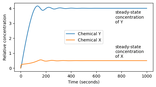
For the parameter values \(k_1=0.1\), \(k_2=0.4\), \(k_3=0.1\) and \(k_4=0.2\), the system results in decaying oscillations of the concentrations \(X\) and \(Y\). Over time the system reaches equilibrium and the values of \(X\) and \(Y\) reach a steady state. The figure below shows the results of the simultion with initial condtions \(X[0] = Y[0] = 0\).
1. Assuming the initial concentrations are zero, run the simulation with the parameters above for \(1000\) time steps. Plot \(X\) and \(Y\) on the same figure, as below.
2. Assuming that the system has reached a steady state after 1000 timesteps, we can define the steady-state concentrations to be \(X_{1000}\) and \(Y_{1000}\). Determine the steady-state values of \(X\) and \(Y\).
3. Write a function steady_state_X(k1, k2, k3, k4) which runs the simulation for the given values of \(k_1\), \(k_2\), \(k_3\) and \(k_4\), then returns the steady-state value of \(X\). Check that it gives the expected value for \(k_1=0.1\), \(k_2=0.4\), \(k_3=0.1\) and \(k_4=0.2\).
ss_x = steady_state_X(0.1, 0.4, 0.1, 0.2)
print(ss_x) # should print the expected value
4. Determine the steady-state value of X for \(k_1=0.1\), \(k_2=0.4\), \(k_3=0.1\) and a range of values of \(k_4\) between \(0\) and \(0.3\). Plot the results on a graph with \(k_4\) on the x-axis and the steady-state value of \(X\) on the y-axis.
5. Write a function max_X(k1, k2, k3, k4) which returns the peak value of the concentration of X, then (on the same graph as the previous question) plot the peak concentration of X for \(k_4\) between \(0\) and \(0.3\). (Use the numpy function np.max which returns the maximum value of an array).
Exercise 3.14
In this question you will investigate the number of prime numbers below a number \(n\) (recall a prime number is a number divisible only by 1 and itself).
You will need to use Boolean variables which are variables that take the logical values True or False. For example, the following function divisible_by_two returns the Boolean value True if its argument is divisible two, and False otherwise.
def divisible_by_two(n):
    if n % 2 == 0:
        return True
    else:
        return False

k = 5
if divisible_by_two(k):
    print(k, "is even")
else:
    print(k, "is odd")
Write a function
is_divisible(n, m)which returnsTrueifnis divisible bym, and otherwise returnsFalse.Write a function
is_prime(n)which returnsFalseifnis divisible by any integer between2andn-1, and otherwise returnsTrue.Write a function
number_of_primes(n)which returns the number of prime numbers less than or equal ton[NB 1 is not a prime number].Draw a graph with
non the x-axis and the number of primes less than or equal tonon the y-axis.
Exercise 3.15
A solid of revolution is a three-dimensional figure contstructed by rotating a curve about a straight line. We can estimate the volume of a solid of revolution by dividing it into a sequence of stacked discs and summing the volume of each.
A sphere of radius \(R\) is formed by rotating the curve \(y = \sqrt{R^2 - x^2}\) around the x-axis between \(-R\) and \(R\).
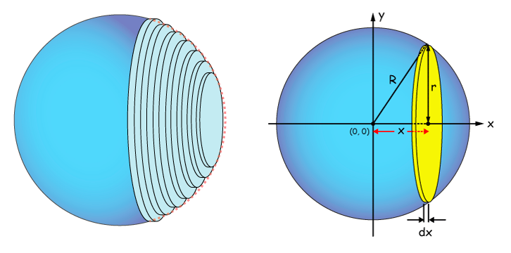
Use the following steps to estimate the volume of a sphere of radius 1.
Write a function
vol_disc(R, x, dx)which returns the volume of the disc centred at positionxwith thicknessdx.Estimate the volume of a sphere of radius 1 by dividing the figure into 10 discs equally spaced between
-1and1[use a value of 3.14159 for \(\pi\)].Write a function
sphere_vol(R, n)which returns the estimate of the volume of a sphere of radiusRcalculated by dividing it intondiscs.The estimate should get more accurate as we increase
n. We can estimate the accuracy by calculating the difference betweensphere_vol(R, n)andsphere_vol(R, n-1). ForR = 1, how large doesnneed to be so that difference between consecutive estimates is less than \(10^{-4}\)?