4.4. Exercises

Exercise 4.12

Downsampling is the process of reducing the size of an image. For example, Downsampling by a factor of 2 would reduce a 10 by 10 image to a 5 by 5 image. One way to do this is to divide the image into 2 x 2 blocks and calculate the average of each block as in Fig. 4.9.

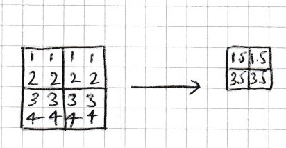
Fig. 4.9 Downsampling a 4 by 4 array by a factor of 2 by averaging 2 by 2 blocks.

1. Write code which downsamples the falling cat image by a factor of 2.

2. Write a function downsample(x, k) which downsamples the array x by a factor k. Test your function against the falling cat image for various values of k.

Upsampling is the reverse process. For example, upsampling by a factor of 2 would increase a 10 by 10 image to a 20 by 20 image. This can be achieved by repeating each element in 2 by 2 blocks as in Fig. 4.10.

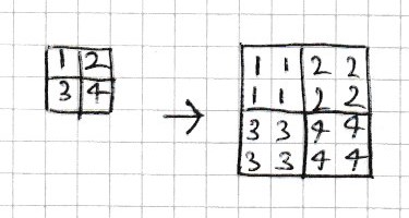
Fig. 4.10 Upsampling a 4 by 4 array by a factor of 2 by repeating each element in 2 by 2 blocks.

3. Write a function upsample(x, k) which upsamples the array x by a factor k. Test your function against the falling cat image for various values of k.

Scalar Fields

A scalar field is a mapping which associates a number with points in space. Examples of scalar fields area atmospheric pressure (measured in millibars) of points in a geographical area, or the temperature (in Kelvin) of points in a 3 dimensional solid body.

Suppose we have a 2-dimensional scalar field given by the following formula:

\[\begin{split} \begin{align} f(x, y) = \begin{cases} \exp(-y^2) & \text{if} -1.5 < x < 1.5 \\ 0 & \text{otherwise.} \end{cases} \end{align} \end{split}\]

Exercise 4.13

Write a function height(x, y) which returns the value of \(f\) evaluated at position \(x, y\).

def height(x, y):
    # calculate result
    
    return result

# check the function works
h = height(0, 0)
print(h) # should print 1

h = height(-2, 0)
print(h) # should print 0

Check that your function works for the two cases above, and write a third test case of your choice.

Exercise 4.14

Create a 10 by 10 numpy array z which contains the values of the scalar field in the region \(-2 < x < 2\) and \(-2 < y < 2\).

N = 10
z = np.zeros((N, N))

x_array = np.linspace(-2, 2, N)
print("x_array:", x_array)

# create y_array for the y values,
# then use nested for loops to calculate values
# of the scalar field in array z

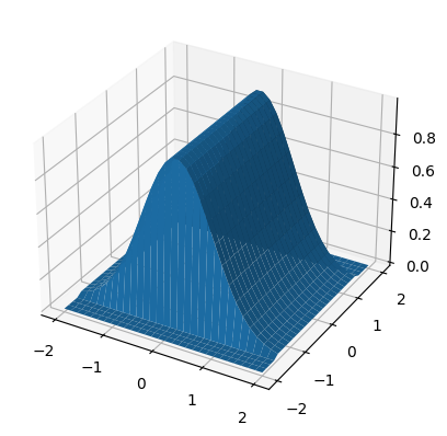
# Use imshow to display the array z as a 2d image

Check that your resulting image agrees with the surface plot shown above.

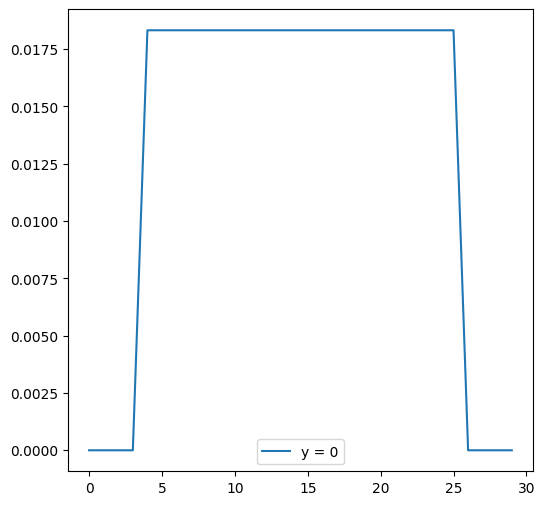
We can investigate the scalar field by taking cross sections for fixed values of \(x\) or \(y\).

cross_section_0 = z[:,0]
print(cross_section_0)

plt.figure(figsize=(6,6))
plt.plot(cross_section_0, label = "y = 0")
plt.legend()

[0.         0.         0.         0.         0.01831564 0.01831564
 0.01831564 0.01831564 0.01831564 0.01831564 0.01831564 0.01831564
 0.01831564 0.01831564 0.01831564 0.01831564 0.01831564 0.01831564
 0.01831564 0.01831564 0.01831564 0.01831564 0.01831564 0.01831564
 0.01831564 0.01831564 0.         0.         0.         0.        ]

<matplotlib.legend.Legend at 0x1da7d77f708>

Exercise 4.15

Plot a graph showing three cross-sections for fixed \(x\), and another graph with three cross-sections for fixed \(y\). You may choose the values of \(x\) and \(y\).

Exercise 4.16

The file pressure_2d.txt contains the pressure (in millibars) in a 2-dimensional square region. Download the file then use the function np.loadtxt to load the data into an array.

Use the techniques you have learnt to investigate the scalar field defined by this data. How many local maxima (peaks) and minima (troughs) are there? What are there co-ordinates and what is the value of the pressure at these points?