2.2. Modelling Change

Python Libraries

The standard Python language is very extensive, containing a wide range of built-in data types and functions, some of which we looked at last week. In addition, we can access an ever-growing collection of Python code libraries. A library is a package of pre-built code that provides useful functions to extend the standard Python library. Probably the two most useful libraries for scientists are numpy (for numerical computing) and matplotlib (for plotting graphs).

Importing Libraries

To access numpy the numpy library we first have to import it using the import keyword.

import numpy as np

This line instructs Python to load the library called numpy and give it the prefix np. Once we have executed this line of code we can access the many numpy data types prefixed by np..

Let’s use numpy to calculate the square-root of two.

x = np.sqrt(2)

print("The square root of 2 is", x)

The square root of 2 is 1.4142135623730951

Note

We can choose any prefix we like, but it is standard (in this course and elsewhere) to always use the prefix np. We will include the line

import numpy as np

at the top of every Python notebook from now on!

See the online documentation for the many mathematical functions and constants defined by numpy.

Exercise 2.1

Import the numpy library and use it to calculate

\[\cos(3\pi/2).\]

Solution to Exercise 2.1

import numpy as np

x = np.cos(3 * np.pi / 2)

print("cos(3 pi/2) = ", x)

This is not exactly 0 - this is okay! This happens because the calculation is done using something called ‘floating point arithmetic’.

Note

You only need to import each library once in your notebook. It is customary to gather your import statements together at the top of the file.

import numpy as np
import matplolib.pyplot as plt

# the rest of your code below

numpy Arrays

An array is a Numpy data type that stores a sequence of values. For example, suppose we have the following data representing five years’ population data:

populations = np.array([12, 25, 54, 102, 206])
print(populations)

[ 12  25  54 102 206]

Each element in an array has an index which identifies its position. We can access an array element by following the variable name with square brackets and the index:

initial_pop = populations[0]
year_3_pop = populations[2]

print("Initial population:", initial_pop)
print("Population in year 3:", year_3_pop)

Initial population: 12
Population in year 3: 54

Note

Arrays are indexed starting from 0, so the first element of array x is x[0], the second is x[1] and so on. If an array has n elements, then the last element is at index n - 1.

Likewise, we can update individual array elements. Suppose we would like to change the value of the 3rd element:

populations[2] = 100
print(populations)

[ 12  25 100 102 206]

Exercise 2.2

Use np.array to create an array with the following values 1, 1, 2, 3, 6, 8.

Change the value of the element at index position 4 from 5 instead of 6.

Solution to Exercise 2.2

fib = np.array([1, 1, 2, 3, 6, 8])
print(fib)

# 5th element is at index (5-1)
fib[4] = 5 
print(fib)

Creating Numpy Arrays

Above, we created an array using the np.array function. Other ways to create an array include the functions np.zeros and np.linspace.

z = np.zeros(6) # Create an array of 6 zeros
print(z)

[0. 0. 0. 0. 0. 0.]

Use np.linspace(a, b, num) to generate num evenly spaced numbers between a and b:

z = np.linspace(0, 1, 4)
print(z)

[0.         0.33333333 0.66666667 1.        ]

Exercise 2.3

Use np.linspace to create an array with the following values:

[0., 0.25, 0.5, 0.75, 1.]

Solution to Exercise 2.3

The array contains 5 numbers so num = 5; it starts at 0 and ends at 1 so we need:

z = np.linspace(0, 1, 5)
print(z)

for Loops

A for loop is used to iterate over a sequence of values. The simplest form of the for statement is to iterate over a range of n integer values. For example, the following code will execute the indented statements once for each integer from 0 to 4:

for i in range(5):
    print("i =", i)

i = 0
i = 1
i = 2
i = 3
i = 4

The variable i is called the iterator variable and is updated during each iteration. The range function specifies the sequence of integer values that the loop variable will take.

syntax	result
range(n)	a sequence from 0 to n - 1
range(a, n)	a sequence from a to n - 1
range(a, n, step)	a sequence from a to n - 1 in steps of step

For example, the following code loops over the integers from 1 to 10 in steps of 2.

for i in range(1, 10, 2):
    print("i =", i)

i = 1
i = 3
i = 5
i = 7
i = 9

Exercise 2.4

Write a for loop which prints the following:

i = 2
i = 5
i = 8
i = 11

Solution to Exercise 2.4

The first value is 2, so a = 2; the final value is 11 so n - 1 = 11, therefore n = 12; the values increase in steps of 3 so step = 3, so we need:

for i in range(2, 12, 3):
    print("i =", i)

Plotting using Matplotlib

Suppose we have collected the following data which we would like to plot on a line graph.

Time (s)	0.1	0.2	0.3	0.4	0.5	0.6	0.7
Distance (m)	2.5	2.6	3.4	4.1	4.5	5.1	5.2

We we plot graphs using a Python library called matplotlib.pyplot. First import the library with the prefix plt and create an array of distance values.

import matplotlib.pyplot as plt

dis = np.array([2.5, 2.6, 3.4, 4.1, 4.5, 5.1, 5.2])

Next we use the function plt.figure to create a figure of suitable dimensions and the function plt.plot to display the array dis as a line graph.

plt.figure(figsize=(4,4)) # create figure of size 4 by 4 inches
plt.plot(dis) # plot a line graph

[<matplotlib.lines.Line2D at 0x14627241a88>]

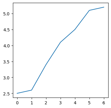
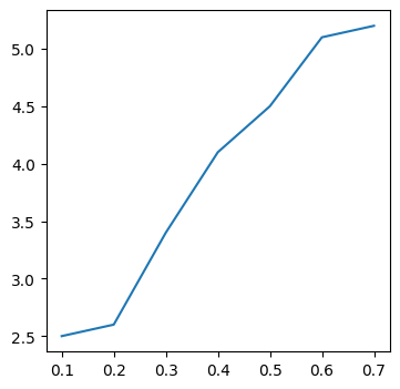
Notice that the data points are plotted at x-coordinates 0 ... 6. To use the actual time values, we need to create a second array time and pass both arrays to the function plt.plot.

dis = np.array([2.5, 2.6, 3.4, 4.1, 4.5, 5.1, 5.2])
time = np.linspace(0.1, 0.7, 7)

plt.figure(figsize=(4,4))
plt.plot(time, dis)

[<matplotlib.lines.Line2D at 0x14627548388>]

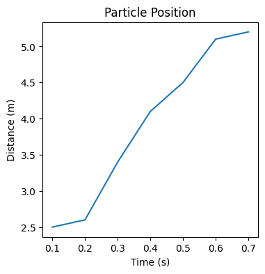
Finally, we add a title and axis labels using functions plt.xlabel, plt.ylabel and plt.title.

plt.figure(figsize=(4,4)) 
plt.plot(time, dis)
plt.xlabel("Time (s)") # add an x-axis label
plt.ylabel("Distance (m)") # add a y-axis label
plt.title("Particle Position") # add a figure title

Text(0.5, 1.0, 'Particle Position')

Exercise 2.5

Plot the following data on a line graph. Include axis labels and a suitable title.

Time (days)	5	10	15	20	25	30
Mass (kg)	110	112	115	120	130	151

Solution to Exercise 2.5

The time data contains 6 evenly-spaced time points starting at 5 and ending at 30, so we can use np.linspace to create the array. The mass data is not a straightforward sequence, so it is easier to just hard code the array.

# record data
time = np.linspace(5, 30, 6)
mass = np.array([110, 112, 115, 120, 130, 151])

# create the figure
plt.figure(figsize=(4,4)) 
plt.plot(time, mass)
plt.xlabel("Time (days)") # add an x-axis label
plt.ylabel("Mass (kg)") # add a y-axis label
plt.title("Mass vs time") # add a figure title