Solutions#
import numpy as np
import matplotlib.pyplot as plt
Solution to Exercise 2.6
The updated code is:
x = np.zeros(5)

x[0] = 10
print("x:", x)

for i in range(5):
    x[i+1] = x[i] + 0.1*x[i]

print("x:", x)
x: [10. 0. 0. 0. 0.]
---------------------------------------------------------------------------
IndexError                                Traceback (most recent call last)
~\AppData\Local\Temp\ipykernel_828\3670759407.py in <module>
      5
      6 for i in range(5):
----> 7     x[i+1] = x[i] + 0.1*x[i]
      8
      9 print("x:", x)

IndexError: index 5 is out of bounds for axis 0 with size 5
If we try and run this we see IndexError: index 5 is out of bounds for axis 0 with size 5.
When we increase the upper limit to \(5\) the final value that is passed through the for loop is i = 4.
Remember that arrays are indexed from \(0\), so x[n] will try to access the (n+1)th element of x.
So when i = 4 the line x[i+1] = x[i] + 0.1*x[i] looks for the element of x at index \(5\), which is the \(6\)th element of x.
But x only has \(5\) elements! So Python is warning us that we are trying to access an element of an array that does not exist - i.e. it is out of bounds.
Solution to Exercise 2.7
First we need to extend the for loop from above. To get \(x_{16}\) we will need to calculate 17 terms of the sequence - remember that the first term is \(x_0\).
x = np.zeros(17)

x[0] = 10

for i in range(16):
    x[i+1] = x[i] + 0.1*x[i]

print("x[16]:", x[16])
x[16]: 45.94972986357215
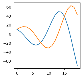
Solution to Exercise 2.8
x = np.zeros(20)
x[0] = 10

# create array y and set initial value
y = np.zeros(20)
y[0] = 10

for i in range(19):
    x[i+1] = x[i] - 0.5 * y[i]

    # set value of y[i+1]
    y[i+1] = y[i] + 0.4 * x[i]

plt.figure(figsize=(3,3))
plt.plot(x)

# plot y on the SAME graph
plt.plot(y)
[<matplotlib.lines.Line2D at 0x2af3bf7ec08>]
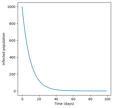
Solution to Exercise 2.9
\(I_0 = 1000\)
\(I_1 = I_0 - 0.1*I_0 = 1000 - 100 = 900\)
\(I_2 = I_1 - 0.1*I_1 = 900 - 90 = 810\)
\(I_3 = I_2 - 0.1*I_2 = 810 - 81 = 729\) and so on…
n_days = 100

I = np.zeros(n_days)

I[0] = 1000

for i in range(n_days - 1):
    I[i+1] = I[i] - 0.1 * I[i]

plt.figure(figsize=(5,5))
plt.plot(I)
plt.xlabel("Time (days)")
plt.ylabel("Infected population")
Text(0, 0.5, 'Infected population')
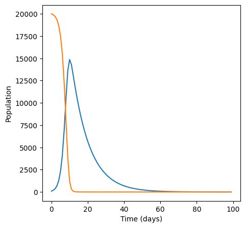
Solution to Exercise 2.10
# set up variables and arrays
n_days = 100
a = 0.1
b = 0.00005
S = np.zeros(n_days)
I = np.zeros(n_days)

# initialise the variables
S[0] = 20000
I[0] = 100

# implement equations
for i in range(n_days - 1):
    S[i+1] = S[i] - (b * S[i] * I[i])
    I[i+1] = I[i] + (b * S[i] * I[i]) - (a * I[i])

plt.figure(figsize=(5,5))
plt.plot(I)
plt.plot(S)
plt.xlabel("Time (days)")
plt.ylabel("Population")
Text(0, 0.5, 'Population')
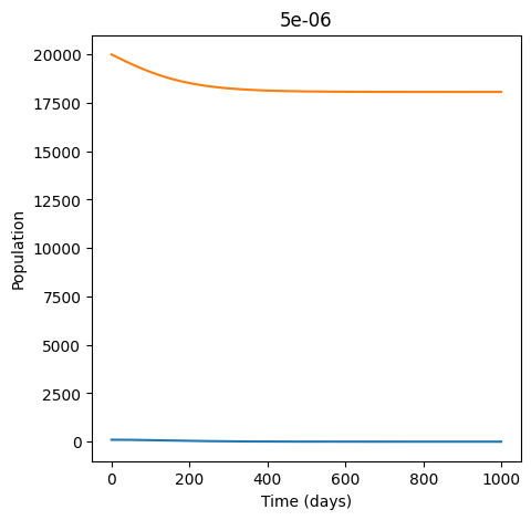
Solution to Exercise 2.11
By experimenting with values of \(b\), you should find that the epidemic disappears somewhere between 0.000005 and 0.000006. To see this you have to increase the value of n_days because the peak gets later as it gets lower.
# set up variables and arrays
n_days = 1000
a = 0.1
b = 0.000005
S = np.zeros(n_days)
I = np.zeros(n_days)

# initialise the variables
S[0] = 20000
I[0] = 100

# implement equations
for i in range(n_days - 1):
    S[i+1] = S[i] - (b * S[i] * I[i])
    I[i+1] = I[i] + (b * S[i] * I[i]) - (a * I[i])

plt.figure(figsize=(5,5))
plt.plot(I)
plt.plot(S)
plt.xlabel("Time (days)")
plt.ylabel("Population")
plt.title(b) # add title so we know what value we are currently looking at
Text(0.5, 1.0, '5e-06')
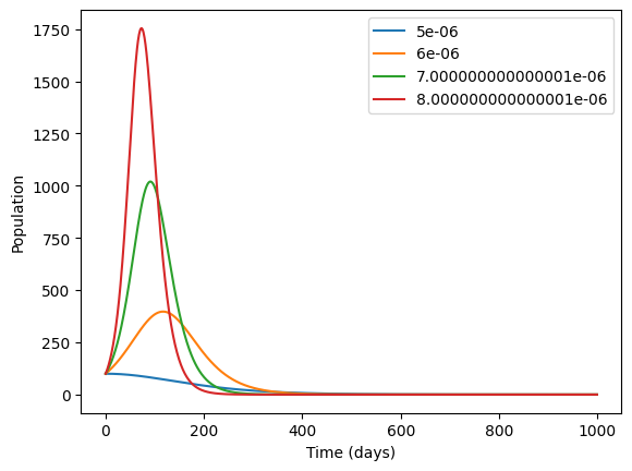
One way to plot multiple solutions on the same plot is to use a loop as below. Note that we have also added a legend.
# set up variables and arrays

for k in range(4):

    b = 0.000001 * k + 0.000005

    n_days = 1000
    a = 0.1

    S = np.zeros(n_days)
    I = np.zeros(n_days)

    # initialise the variables
    S[0] = 20000
    I[0] = 100

    # implement equations
    for i in range(n_days - 1):
        S[i+1] = S[i] - (b * S[i] * I[i])
        I[i+1] = I[i] + (b * S[i] * I[i]) - (a * I[i])


    plt.plot(I, label = b)


plt.xlabel("Time (days)")
plt.ylabel("Population")
plt.legend()
<matplotlib.legend.Legend at 0x2af43a20c08>
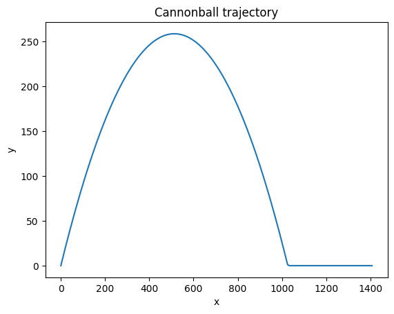
Solution to Exercise 2.12
n = 200
g = 9.81
dt = .1

theta = np.pi / 4
s = 100


x = np.zeros(n)
y = np.zeros(n)
u = np.zeros(n)
v = np.zeros(n)

# initialise the variables
u[0] = np.cos(theta) * s
v[0] = np.sin(theta) * s

# implement equations
for i in range(n - 1):
    x[i+1] = x[i] + u[i] * dt
    y[i+1] = y[i] + v[i] * dt
    if y[i+1] < 0:
        y[i+1] = 0 # set y to zero if negative
    u[i+1] = u[i]
    v[i+1] = v[i] - g * dt

plt.plot(x, y)
plt.xlabel("x")
plt.ylabel("y")
plt.title("Cannonball trajectory")
Text(0.5, 1.0, 'Cannonball trajectory')