5.2. Cellular Automata

Advanced Plotting

The plotting library matplotlib is capable of producing quite sophisticated and professional-looking figures. The online documentation contains a number of examples including demonstration code.

One of the most useful techniques allows you to include multiple plots in a single Figure. To use it we have to use Matplotlib’s ‘explicit’ interface, where we create figure and axis objects and then call methods on them using an ‘object-oriented’ style syntax. A full understanding of this style of programming is out of the scope of this course, but you should nevertheless be able to make use of this functionality by adapting the examples below.

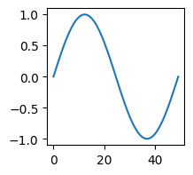
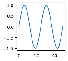
First let’s take an example using Matplotlib’s ‘implicit’ (conventional) syntax to plot the functions \(\sin(x)\) and \(\sin(2x)\) on two separate figures.

import numpy as np
import matplotlib.pyplot as plt

t = np.linspace(0, 2 * np.pi)
x1 = np.sin(t)
x2 = np.sin(2*t)

plt.figure(figsize=(2,2))
plt.plot(t, x1)

plt.figure(figsize=(2,2))
plt.plot(t, x2)

[<matplotlib.lines.Line2D at 0x244d47ecb08>]

Next we will use Matplotlib’s explicit interface to plot the two curves on one figure. In Matplotlib, a Figure object represents a graphical container within which we can plot onto a number of Axis objects. Up to now, our figures have each contained exactly one axis. Now we will see how to create figures containing multiple axes.

The function plt.subplots create a Figure object and a collection of Axis objects. plt.subplots(n, m) creates a figure comprising an n by m grid of axes.

Instead of plt.plot we use axes[i].plot where i is the index of the axis we would like to plot onto.

fig, axes = plt.subplots(1, 2, figsize=(4, 2))
axes[0].plot(x1)
axes[1].plot(x2)

[<matplotlib.lines.Line2D at 0x244d40ede08>]

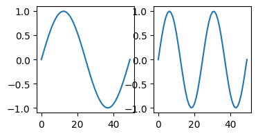
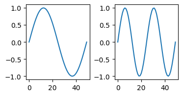
Unfortunately, Matplotlib doesn’t always do a good job of arranging the axes within the figure! You might need to tweak the layout using Matplotlib’s vast library of functions. Here, we use the function subplots_adjust to add white space between the axes.

fig, axes = plt.subplots(1, 2, figsize=(4, 2))
axes[0].plot(x1)
axes[1].plot(x2)
fig.subplots_adjust(wspace=0.4)

Alternatively, we might like to remove the axes entirely.

fig, axes = plt.subplots(1, 2, figsize=(4, 2))
axes[0].plot(x1)
axes[1].plot(x2)

axes[0].axis("off")
axes[1].axis("off")

(-2.45, 51.45, -1.0994348378207568, 1.0994348378207568)

Exercise 5.1

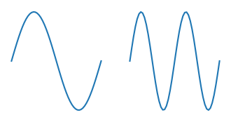
Use a for loop to plot \(\sin(nx)\) for \(n=1 \ldots 10\) on a single figure as below.

Solution to Exercise 5.1

t = np.linspace(0, 2 * np.pi, 100)
N = 10

fig, axes = plt.subplots(1, N, figsize=(N, 1))
for i in range(N):
    axes[i].plot(np.sin(t * (i+1)))
    axes[i].axis("off")

Multi-dimensional Arrays

Numpy arrays come is various types, shapes and sizes. So far we have studied 1-dimensional and 2-dimensional arrays. Elements of a 1-d array are access by one index variable:

a1 = np.array([1, 2, 3, 4])

print(a1[0]) # element at index 0

1
8

On the other hand, 2-d arrays require 2 index variables:

a2 = np.array([[1, 2, 3],
               [4, 5, 6],
               [7, 8, 9]])

print(a2[2, 1]) # element at row 2 column 1

8

Numpy arrays can have as many dimensions as we like. For example, the array in Fig. 5.1 (right) has 3 dimensions.

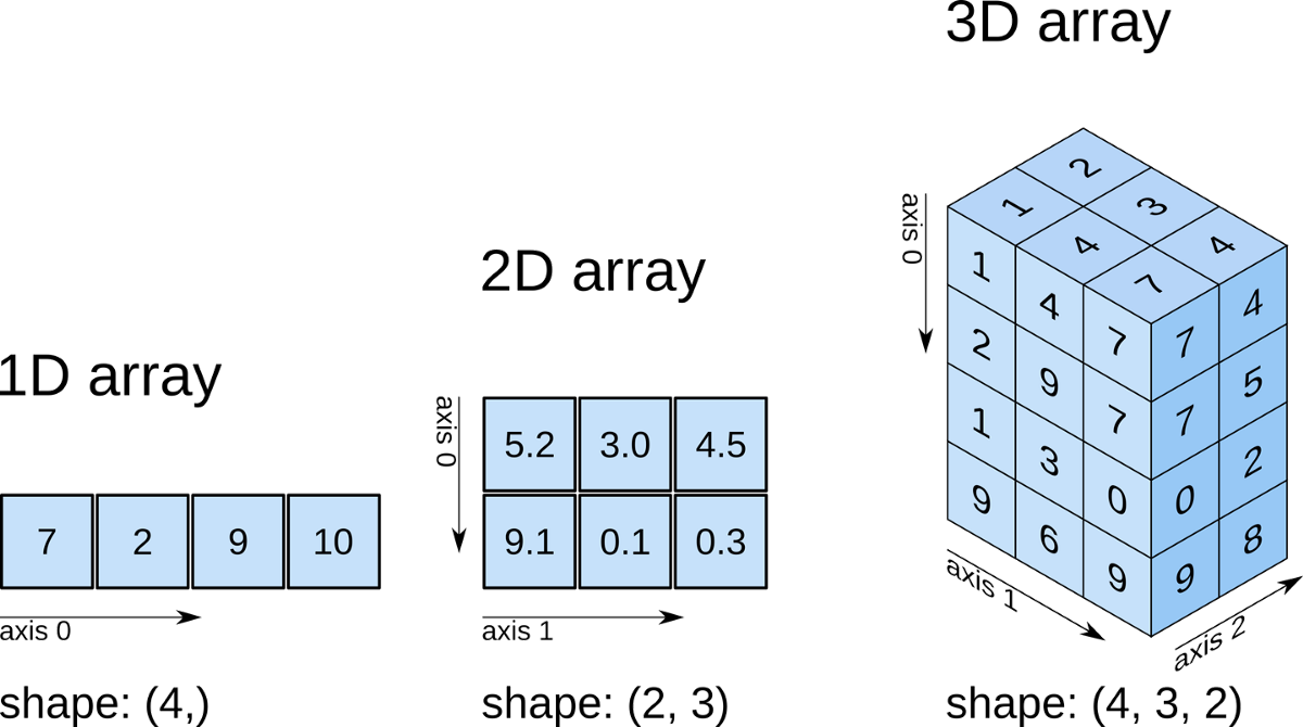
Fig. 5.1 A 1-dimensional array is indexed by 1 coordinates x[i]. A 2-dimensional array is indexed by 2 coordinates x[i,j].A 3-dimensional array is indexed by 3 coordinates x[i,j,k]. In the 3-d array above (right), x[0,2,1] = 4.

We can create this 3d array by stacking 2d arrays together. Notice how it is built from four 3 by 2 arrays each corresponding to a horizontal layer of the array shown in Fig. 5.1 (right).

x = np.array([[[1, 2],
              [4, 3],
              [7, 4]],

              [[2, 0],
              [9, 0],
              [7, 5]],
              
              [[1, 0],
              [3, 0],
              [0, 2]],
              
              [[9, 0],
              [6, 0],
              [9, 8]]])

1

Each element of x is now indexed by three variables:

print(x[0, 2, 1])

4

We can recover the individual 2d arrays using slice notation. The top ‘layer’ of the array is given by:

print(x[0,:,:])

[[1 2]
 [4 3]
 [7 4]]

Exercise 5.2

Use slice notation to obtain the front face and front corner of the array x:

[[1 4 7]
 [2 9 7]
 [1 3 0]
 [9 6 9]]

and

[7 7 0 9]

Solution to Exercise 5.2

print(x[:,:,0]) # front face
print(x[:,2,0]) # front corner