14. Forestry management

Mathematical Bioeconomics: The Mathematics of Conservation., CW Clark

Biological renewable resources, essential to the survival of mankind, are increasingly overexploited by individuals and corporations that often sacrifice long-term economic health and sustainability for short-term gains.

This case study is adapted from a mathematical discussion of forestry management found in a first edition (1976) copy of the above textbook, which is now in its third edition (2010).

Solving the problem requires a combination of techniques studied in this module including finding minima, numeric differentiation, summation of geometric series, curve fitting, plotting, and understanding concepts of relative growth rates.

The problem is to determine the optimal time to harvest a forest resource based on the economic value of timber.

14.1. Without replanting

It is assumed that the timber (wood) value of a tress increases with age up to full maturity. Eventually decay will cause a decline in the tree value, but many commercial tree species continue to grow and increase in value for several hundred years.

We wish to determine the value of cutting down trees at the present time in comparison to the future. Our method will take into account the possibility of interest accrued on a present payment.

Let \(\hat{V}\) denote the present value of a future payment, and let \(V(t)\) denote the commercial value of a tree. Then,

(14.1)\[\begin{equation} \hat{V}=e^{-\delta t}(V(t)-c) \end{equation}\]

where \(c\) is the cost of felling, and \(\delta\) is the annual rate of interest.

Exercise 14.1

Derive a condition for when the value of felling is maximised.

Differentiating the value function:

\[\begin{equation*} \hat{V}^{\prime}=e^{-\delta t}(V^{\prime}-\delta(V-c)) \end{equation*}\]

To maximise \(\hat{V}\) we must ensure that \(\frac{V^{\prime}}{V-c}=\delta\).

---

14.2. With replanting

The basic analysis above neglects the opportunity to replant. When replanting is taken into account we have

(14.2)\[\begin{equation} \hat{V}=e^{-\delta T_1}[V(T_1)-c]+e^{-\delta T_2}[V(T_2-T_1)-c]+e^{-\delta T_3}[V(T_3-T_2)-c]+\dots \end{equation}\]

Assuming that the interest rate will stay constant, the second rotation problem is identical to the first (and so on). We can therefore assume that all rotation periods are equal and so \(T_k=kT\), \(k=1,2,\dots\).

Thus, we may write :

(14.3)\[\begin{equation} \hat{V}=\sum_{k=1}^{\infty}e^{-k\delta T}[V(T)-c]=[V(t)-c]\sum_{k=1}^{\infty}e^{-k\delta T}. \end{equation}\]

The sum is a geometric progression With first term and common difference both equal to \(e^{-\delta T}\). From the formula for the infinite sum we therefore obtain the modified value function:

(14.4)\[\begin{equation} \hat{V}=\frac{V(T)-c}{e^{\delta T}-1} \end{equation}\]

Exercise 14.2

Show that the modified value function is maximised for

(14.5)\[\begin{equation} \frac{V^{\prime}}{V-c}=\frac{\delta}{1-e^{-\delta T}} \end{equation}\]

This is the Faustmann formula.

Differentiating gives:

(14.6)\[\begin{equation} \hat{V}^{\prime}=\frac{(e^{\delta T}-1)V^{\prime}-(V-c)\delta e^{\delta T}}{(e^{\delta T}-1)^2} \end{equation}\]

The result is then obtained by setting \(\hat{V}^{\prime}=0\).

---

14.2.1. Interpretation

Because \(1-e^{-\delta T}<1\), taking rotation into account leads to a decrease in the age of cutting.

The Faustmann formula can be understood by rearrangement to:

(14.7)\[\begin{equation} V^{\prime}=\delta(V-c)+\delta\left(\frac{V-c}{e^{\delta T}-1}\right) \end{equation}\]

• The first term represents the interest earned if revenue from cutting is invested at interest rate \(\delta\)

• The second term represents the rotation aspect of the problem.

14.3. Fitting to data

In the Faustmann formula, \((V-c)\) is the net stumpage value, which can be determined from data tables. We can plot the functions on the left and right side of the formula and calculate their intersection.

Table 14.1 Yield tables for Douglas fir, multiplied by cost (in cents per cubic foot!)

Year	30	40	50	60	70	80	90	100	110	120
\(V-c\)	0	43	143	303	497	650	805	913	1002	1076

Exercise 14.3

Determine the relative growth rate \(V^{\prime}/(V-c)\) and the average yield \((V-c)/T\)

Hint: to estimate \(V^{\prime}\) use the central differences formula

import numpy as np

t=np.arange(30,121,10)
y=np.array([0,43,143,303,497,650,805,913,1002,1076]) #y=V-c

gr=(y[2:]-y[0:-2])/(t[2:]-t[0:-2])   #growth rate
relgr=gr/(y[1:-1])                   #relative gr            
print(100*relgr)

Year \(T\)	30	40	50	60	70	80	90	100	110	120
net stump val	0	43	143	303	497	650	805	913	1002	1076
Rel gr rate %	-	16.6	9.1	5.8	3.5	2.4	1.6	1.1	0.8	0
Avg yield	0	1.08	2.86	5.05	7.10	8.12	8.94	9.13	9.11	8.97

Exercise 14.4

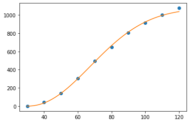
Fit a Weibull function to the net stumpage value. The Weibull function is given by

(14.8)\[\begin{equation} w(t) = 1-e^{-(t/k)^s} \end{equation}\]

Hint: The data need to be transformed to the range [0,1] on both axes to perform the fit, and then the inverse transform needs to be performed. It’s worth it though, as the data fit very nicely!

import matplotlib.pyplot as plt

# plot the data
plt.plot(t,y,'o')

# function to fit, with unknown parameters
def func(t,k,s):
  return 1-np.exp(-(t/k)**s)

#scale t,y to [0,1]
tscl=(t-30)/90
yscl=y/np.max(y)

# fit the function
from scipy import optimize
coeffs=optimize.curve_fit(func,tscl,yscl)[0]

#generate fitted curve
tt=np.linspace(30,120)
yy=np.max(y)*func((tt-30)/90,*coeffs)
plt.plot(tt,yy)
plt.show()

14.4. Optimal harvesting

Using the fitted Weibull function, we can produce a figure illustrating the intersections of the left and right sides of the Faustmann formula for different values of the interest rate \(\delta\).

# Left-hand side of Faustmann formula
T=np.linspace(1,120)
for d in [0.001,0.05,0.1,0.15]:
  plt.plot(T,d/(1-np.exp(-d*T)),'k')
  plt.text(100, max([0.015,d+0.005]), '$\delta=$ %0.2f' % d)

# Right-hand side of Faustmann formula (data)
plt.plot(t[1:-1],relgr,'o')

# Right hand side of Faustmann formula (function)
plt.plot(tt[0:-1],np.diff(yy)/np.diff(tt)/yy[0:-1])

plt.xlim([0,120])
plt.ylim([0,0.20])
plt.show()

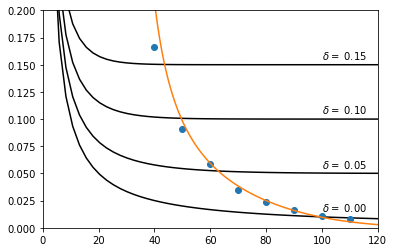
Fig. 14.1 Graphical determination of the optimal rotation for different interest rates \(\delta\)

The intersections give the optimal rotation age (years) for different values of the discount. To numerically locate the intersections we can find where the difference between the two datasets representing the curves is smallest.

tt=np.linspace(30,120,1000)             #ensure plenty of data points
yy=np.max(y)*func((tt-30)/90,*coeffs)   #(V-c)
LHS=np.diff(yy)/np.diff(tt)/yy[0:-1]    #V'/(V-c)

def optrot(d):
  RHS=d/(1-np.exp(-d*tt[0:-1]))         #d/(1-exp(-dT))
  minfun=np.abs(LHS-RHS)                #we want where LHS-RHS=0
  idx=np.argmin(minfun)                 #find data point minimum
  return [tt[idx],yy[idx]/tt[idx]]      #return T, (V-c)/T

dvals=[0.0001,0.03,0.05,0.07,0.1,0.15,0.20]
[print(optrot(d)) for d in dvals];

Annual discount \(\delta\)	0.00	0.03	0.05	0.07	0.10	0.15	0.20
Optimal rotation age T (yr)	99	73	63	56	50	44	40
Avg annual yield	9.23	7.42	5.61	4.16	2.72	1.48	0.91