7. Rates of change

The Newton-Leibniz Calculus Controversy

The philosophical and political dimension of the debate between Leibniz and Newton should not escape our attention. They disagreed over issues concerning the foundations of the calculus: Newton was convinced of the superiority of his method of limits over Leibniz’s mathematical practice where infinitesimals occurred. They were divided over physical questions such as the nature of gravity, time and space, atoms and the void, as well as the issue of which quantities are properly conserved by the laws of nature. In short, they were not just mathematical opponents: they were philosophical enemies as well.

In this chapter we introduce the concept of a derivative and some standard results. After completing this chapter you should be able to:

• obtain a numeric estimate of the derivative using data points representing a curve

• differentiate simple functions by hand

• Use sympi to obtain analytic derivatives of more difficult functions

• apply the sum, product, reciprocal and chain rules for differentiation.

• find the equation of the tangent at a given point on a curve

• find and classify stationary points of functions

7.1. Motivation

Much of what we do in the natural sciences is concerned with studying the relationships between variables. We often consider the effect of changing one variable upon the other, which we call the dependent variable. For instance, we might consider how changing CO2 levels affect global temperatures, how student debt grows over time, or the way that a drug binds to biological receptors as a function of the chemical concentration.

In such problems it is natural to find ourselves discussing the rate of change of the dependent variable, which can be represented graphically by the slope of the function curve. Indeed, when we looked at student debt we saw that characterising the growth rate is a fundamental idea of the exponential model.

We also use these ideas very naturally in our day-to-day activities - such as guesstimating how long a bathtub will take to fill at a given rate, how long a cup of tea will take to cool, or how long it will take to reach our journey destination at the current speed. In many scenarios a back-of-an-envelope calculation can be made by assuming a constant rate of change to provide a useful result. To do this for a nonlinear model function we require a method to estimate the rate of change at each point on the curve.

Exercise 7.1

You are studying a new blood pressure drug. At a dose of 5mg the slope of the dose-response curve is -2 mmHg/mg. Approximately how much would a patient’s blood pressure change if the drug dose was increased to 5.1mg?

According to the information given in the question, blood pressure decreases by 2mmHg per mg increase in dose. Thus, for a 0.1mg increase in dose we expect blood pressure to decrease by 0.2mmHg. We can write out the calculation mathematically as follows:

Let \(R\) be the response and \(D\) be the dose, and let \(\Delta R,\ \Delta D\) represent changes in these quantities. According to the information given in the question,

\[\begin{equation*} \frac{\Delta R}{\Delta D}=-2\frac{\text{mmHg}}{\text{mg}}. \end{equation*}\]

Taking \(\Delta D=0.1\text{mg}\) then gives

\[\begin{equation*} \Delta R = -2 \frac{\text{mmHg}}{\text{mg}}(0.1\text{mg})=-0.2\text{mmHg}. \end{equation*}\]

The blood pressure would decrease by 0.2mmHg.

Here, we treated the slope of the dose-response curve as constant, which is usually a reasonable approximation when looking at small changes.

---

7.2. Estimating slope of a curve

We can obtain an approximation to a curve by joining up a set of points with straight lines. This is known as a “linear interpolation”. It is the approach we used to plot curves in the previous sections of these notes. For example, the following code produces a plot of \(y=x^2\), using 30 data points connected by straight lines.

import matplotlib.pyplot as plt
import numpy as np

n=30 # number of data points
x=np.linspace(-3,3,n)
y=x**2

plt.plot(x,y)
plt.show()

In the animation below this basic code has been adapted to illustrate how the interpolation appears smoother and more representative of the function as we use a greater number of datapoints in the interval.

Once Loop Reflect

We can use the linear interpolation to estimate the slope of the curve at each datapoint. The formula can be written mathematically by labelling the points as

\[\begin{equation*} (x_k,y_k), \qquad k=1,2,\dots n. \end{equation*}\]

The slope of each line segment is then given by

\[\begin{equation*} s_k = \left[\frac{\Delta y}{\Delta x}\right]_k = \frac{y_{k+1}-y_k}{x_{k+1}-x_k}. \end{equation*}\]

The code below provides an implementation of the formula for a given set of points to find an estimate of the slope at the values where it is available.

def fdiff(x,y):
    ydiffs = y[1:]-y[:-1]
    xdiffs = x[1:]-x[:-1]
    return ydiffs/xdiffs

Exercise 7.2

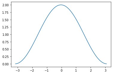
Plot a numeric estimate of the slope at each point in the interval \(-\pi\leq x \leq \pi\) for the function

\[\begin{equation*} y(x)=\sin(x)+x \end{equation*}\]

Notice that with \(n\) data points we can only find the slope at the first \((n−1)\) points, because the forward projection of the function at the final point is not known. If we wish to obtain the slope at \(x_n\), we require the exterior value \((x_{n+1},y_{n+1})\).

import matplotlib.pyplot as plt
import numpy as np

x=np.linspace(-np.pi,np.pi,100)
y = np.sin(x)+x

yd=fdiff(x,y)
plt.plot(x[0:-1],yd)
plt.show()

7.3. Differentiation principle

Based on our argument that the interpolation is improved when the datapoints are closer together, we can obtain a better numeric estimate of the slope by using more datapoints in the interval.

Analytically, we can obtain the result with infinite precision by taking the limit as \(\Delta x\to 0\). We call the result “the derivative”, and we denote it by

(7.1)\[\frac{\mathrm{d}y}{\mathrm{d}x} = \lim_{\Delta x\to 0}\frac{\Delta y}{\Delta x} =\lim_{\Delta x \to 0}\frac{y(x+\Delta x)-y(x)}{\Delta x}.\]

7.3.1. Polynomials

We can apply the analytic definition above to find the derivatives of polynomials from first principles.

By way of example, let’s consider the function \(y(x)=x^2\). Using the definition we have

\[\begin{align*} \frac{\Delta f}{\Delta x}=\frac{f(x+\Delta x)-f(x)}{\Delta x} &= \frac{(x+\Delta x)^2-x^2}{\Delta x}\\ &=\frac{x^2+2\Delta x+(\Delta x)^2-x^2}{\Delta x}=2x+\Delta x. \end{align*}\]

In the limit,

\[\begin{equation*} \frac{\mathrm{d}y}{\mathrm{d}x} = \lim_{\Delta x\rightarrow 0}\frac{\Delta f}{\Delta x}=2x. \end{equation*}\]

Exercise 7.3

Calculate the derivative of \(y=x^n\) from first principles, where \(n\) is a natural number. (1,2,3,…)

\(y(x+\Delta x) = (x+\Delta x)^n = x^n+nx^{n-1}\Delta x + \mathcal{O}((\Delta x)^2).\)

\(\displaystyle \frac{\Delta y}{\Delta x}=\frac{y(x+\Delta x)-y(x)}{\Delta x} = nx^{n-1}+\mathcal{O}(\Delta x)\)

Therefore, using the definition, \(\displaystyle \frac{\mathrm{d}y}{\mathrm{d}x}=n x^{n-1}.\)

---

7.3.2. Exponentials

For the function \(y=e^x\) we have

\[\begin{equation*} \frac{\Delta y}{\Delta x} = \frac{e^{x+\Delta x}-e^x}{\Delta x} = e^x \left(\frac{e^{\Delta x}-1}{\Delta x}\right). \end{equation*}\]

Recall from our earlier work on exponentials that the natural exponent \(e\) satisfies

\[\begin{equation*} \lim_{\Delta x\rightarrow 0}\frac{e^{\Delta x}-1}{\Delta x}=1 \qquad \implies \quad \frac{\mathrm{d}y}{\mathrm{d}x}=e^x. \end{equation*}\]

7.3.3. Operator notation

We can think of differentiation as an operation that we carry out on a function. With this in mind, we also use the following notation in which \(\mathrm{d}/\mathrm{d}x\) represents the differential operator

(7.2)\[\frac{\mathrm{d}}{\mathrm{d}x}\biggr(y\biggr).\]

This notation can be straightforwardly extended to use for repeated differentiation. For example, the “second derivative” is given by

(7.3)\[\frac{\mathrm{d}}{\mathrm{d}x}\biggr(\frac{\mathrm{d}y}{\mathrm{d}x}\biggr) = \frac{\mathrm{d}^2}{\mathrm{d}x^2}\biggr(y\biggr).\]

Exercise 7.4

Find the second derivative of \(y=x^4\).

\(\displaystyle \frac{\mathrm{d}^2}{\mathrm{d}x^2}\biggr(x^4\biggr)=\frac{\mathrm{d}}{\mathrm{d}x}\biggr(4x^3\biggr)=12x^2.\)

---

In general, the \(n^{\textrm{th}}\) derivative is denoted by \(\frac{\mathrm{d}^n}{\mathrm{d}x^n}\).

7.3.4. Lagrange’s notation

An alternative notation uses a prime mark to denote the derivative in the following manner:

\[\begin{equation*} y^{\prime}(x)=\frac{\mathrm{d}y}{\mathrm{d}x}, \qquad y^{\prime\prime}(x) = \frac{\mathrm{d}^2 y}{\mathrm{d}x^2}, \qquad y^{\prime\prime\prime}(x) = \frac{\mathrm{d}^3 y}{\mathrm{d}x^3}, \qquad \text{etc.} \end{equation*}\]

The dash notation becomes a bit cumbersome for higher derivatives so we write

\[\begin{equation*} f^{(n)}(x)=\frac{\mathrm{d}^n y}{\mathrm{d}x^n}. \end{equation*}\]

7.4. Differentiation rules

The following rules can all be proved from the limit definition

7.4.1. Sum rule:

Taking \(y=u(x)+v(x)\),

(7.4)\[\begin{equation} \frac{\mathrm{d}}{\mathrm{d}x}\biggr(u+v\biggr)=\frac{\mathrm{d}u}{\mathrm{d}x}+\frac{\mathrm{d}v}{\mathrm{d}x}. \end{equation}\]

Exercise 7.5

Use the sum rule to calculate the derivative of \(y=x^3+e^x\)

Taking \(u=x^3\) and \(v=e^x\) gives \(\frac{\mathrm{d}y}{\mathrm{d}x}=3x^2+e^x\).

7.4.2. Product rule:

Taking \(y=u(x)v(x)\),

(7.5)\[\begin{equation} \frac{\mathrm{d}}{\mathrm{d}x}\biggr(uv\biggr)=u\frac{\mathrm{d}v}{\mathrm{d}x}+v\frac{\mathrm{d}u}{\mathrm{d}x}. \end{equation}\]

Exercise 7.6

Use the product rule to calculate the derivative of \(x^3e^x\)

Taking \(u=x^3\) and \(v=e^x\) gives \(\frac{\mathrm{d}y}{\mathrm{d}x}=3x^2 e^x+x^3e^x.\)

7.4.3. Chain rule:

Taking \(y=y(u)\) where \(u=u(x)\),

(7.6)\[\begin{equation} \frac{\mathrm{d}y}{\mathrm{d}x} = \frac{\mathrm{d}y}{\mathrm{d}u}\frac{\mathrm{d}u}{\mathrm{d}x}. \end{equation}\]

Exercise 7.7

Use the chain rule to find the derivative of \(y=e^{x^3}\)

Taking \(u=x^3\) gives \(\frac{\mathrm{d}y}{\mathrm{d}x}=3x^2e^{x^3}.\)

7.4.4. Reciprocal rule:

As a special case of the chain rule we may derive the following result:

(7.7)\[\begin{equation} \frac{\mathrm{d}y}{\mathrm{d}y} = \frac{\mathrm{d}y}{\mathrm{d}x}\frac{\mathrm{d}x}{\mathrm{d}y} \qquad \implies \quad \frac{\mathrm{d}y}{\mathrm{d}x} = 1\biggr/\frac{\mathrm{d}x}{\mathrm{d}y}. \end{equation}\]

Exercise 7.8

Use the reciprocal rule to find the derivative of \(y=\ln(x)\).

Hint: start by rearranging the given equation so that you can use the known result for the derivative of the exponential function.

Rearranging to \(x=e^y\) and differentiating with respect to \(y\) gives

\[\begin{equation*} \frac{\mathrm{d}x}{\mathrm{d}y}=e^{y} \qquad \implies \quad \frac{\mathrm{d}y}{\mathrm{d}x}=\frac{1}{e^y}=\frac{1}{x}. \end{equation*}\]

7.4.5. Difficult derivatives

You can use the symbolic mathematics library sympy to find the derivative of functions in Python if you are not able to differentiate them by hand. The code below gives an example for the derivative of \(y=e^x\sin(x^2)\).

from sympy import *
from sympy.abc import x,y
expr=exp(x)*sin(x**2)
diff(expr, x)

\(\displaystyle 2xe^x\cos(x^2)+e^x\sin(x^2)\)

Exercise 7.9

Could you verify this result by hand, given that the derivative of \(\sin(x)\) is \(\cos(x)\) ?

Let’s first of all label the thing that we want to differentiate:

\[\begin{equation*}y=e^x\sin(x^2).\end{equation*}\]

The dependent variable \(y\) is a product of two terms so we use the product rule.

Taking \(u=e^x\) and \(v=\sin(x^2)\) gives

\[\begin{equation*} \frac{\mathrm{d}y}{\mathrm{d}x}=u\frac{\mathrm{d}v}{\mathrm{d}x}+v\frac{\mathrm{d}u}{\mathrm{d}x}=e^x\frac{\mathrm{d}v}{\mathrm{d}x}+\sin(x^2)e^x. \end{equation*}\]

To differentiate \(v\) we will use the chain rule, since it is a “function of a function”.

Defining \(w=x^2\) so that \(v=\sin(w)\) gives

\[\begin{equation*} \frac{\mathrm{d}v}{\mathrm{d}x}=\frac{\mathrm{d}v}{\mathrm{d}w}\frac{\mathrm{d}w}{\mathrm{d}x}=\cos(w)2x = 2x\cos(x^2). \end{equation*}\]

Substituting this into our earlier expression gives the final result

\[\begin{equation*} \frac{\mathrm{d}y}{\mathrm{d}x}= 2xe^x\cos(x^2)+e^x\sin(x^2). \end{equation*}\]

7.5. Tangent and normal

The equation of a line through point \((x_0,y_0)\) with slope \(m\) is given by

\[\begin{equation*} \frac{y-y_0}{x-x_0}=m \qquad \text{i.e} \qquad y=m(x-x_0)+y_0. \end{equation*}\]

The equation follows directly from the fact that the slope of the line is constant and therefore for any two point \((x,y)\) on the line the ratio \(\Delta y/\Delta x\) is equal to \(m\).

7.5.1. Tangent

The tangent line at a given point \((x_0,y_0)\) on a curve is defined as the line with the same slope as the curve. The equation is therefore given by the following result, in which the notation \([]_{x=x_0}\) means that the enclosed expression is evaluated at \(x=x_0\).

(7.8)\[\begin{equation} \frac{y-y_0}{x-x_0}=m, \qquad m=\left[\frac{\mathrm{d}y}{\mathrm{d}x}\right]_{x=x_0} \end{equation}\]

The code below illustrates how we can use this definition to plot the tangent to the curve \(y=x^2\), using the analytic derivative \(\frac{\mathrm{d}y}{\mathrm{d}x}=2x\).

import matplotlib.pyplot as plt
import numpy as np

# define the function and its derivative

def yfun(x):
  return x**2

def dydx(x):
  return 2*x

# plot the function
x= np.linspace(-3,3,30)
y= yfun(x)
plt.plot(x,y)

# line through the point (x0,y0) with slope m
def line(x0,y0,m):
    x=np.array([-10,x0,10]) #ends and midpoint
    return x,m*(x-x0)+y0

# plot the tangent at specified locations
for x0 in [0.2,1.2]:
  y0=yfun(x0); m=dydx(x0)
  x,y = line(x0,y0,m)
  plt.plot(x,y,'ko--')

#prettify
plt.xlim([-3,3])
plt.ylim([-1,7])
plt.xlabel('x')
plt.show()

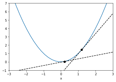
Fig. 7.1 \(y=x^2\) and its tangent at \(x=0.2,\ 1.2\)

Exercise 7.10

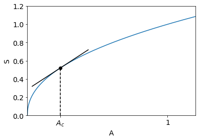
The number of species \(S\) living on an island or habitat fragment of area \(A\) can be modelled as

\[\begin{equation*} S = cA^z, \end{equation*}\]

where \(z > 0\). We can measure area in units that make \(c = 1\). The value of \(z\) is found by data fitting to be approximately 0.45.

Produce a plot of \(S\) and also plot the tangent at the critical value \(A_c\) where

\[\begin{equation*} \left[\frac{\mathrm{d}S}{\mathrm{d}A}\right]_{A=A_c}=1 \end{equation*}\]

Explain the significance of \(A_c\) for biodiversity conservation.

We can find when \(\frac{\mathrm{d}S}{\mathrm{d}A}=1:\)

\[\begin{equation*} 0.45A_c^{-0.55}=1 \quad \Rightarrow \quad A_c=\left(\frac{9}{20}\right)^{20/11}\simeq 0.234 \end{equation*}\]

The tangent equation at the point \((A_c,S_c)\) is given by

\[\begin{equation*} S = (A-A_c)+S_c. \end{equation*}\]

A plot of the habitat equation and tangent at the critical point is shown below. For areas below the critical value, any loss of habitat results in a proportionally greater loss of species.

import matplotlib.pyplot as plt
import numpy as np

# Plot the habitat equation
A = np.linspace(0,1.2,1000)
plt.plot(A, A**0.45)

# Plot the critical point
Ac = (1/0.45)**(-1/0.55)
Sc = Ac**0.45
plt.plot(Ac,Sc,'ko')
plt.plot([Ac,Ac],[0,Sc],'k--')

# Plot the tangent
T=np.array([-0.2,0.2]) +Ac  #end values
plt.plot(T,(T-Ac)+Sc,'k')

# Prettify
plt.xlabel('A')
plt.ylabel('S')
plt.xlim([0,1.2])
plt.ylim([0,1.2])
plt.xticks([Ac,1],labels=["$A_c$",1])
plt.show()

7.5.2. Normal

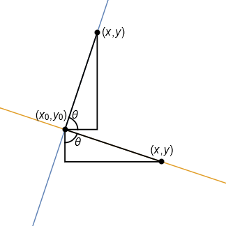
The gradient of the normal (perpendicular) line to the tangent is \(-1/m\). The equation of the normal line is therefore given by

(7.9)\[\begin{equation} \quad \frac{y-y_0}{x-x_0}=-\frac{1}{m} \qquad m=\left[\frac{\mathrm{d}y}{\mathrm{d}x}\right]_{x=x_0} \end{equation}\]

The justification for this result is illustrated below, using the similarity of the two illustrated triangles.

Let \(\theta\) be the illustrated angle and define \(m=\tan(\theta)\), representing the gradient of the blue line.

The equation of the perpendicular line is therefore given by

\[\begin{equation*} m= \frac{x-x_0}{-(y-y_0)} \implies \frac{y-y_0}{x-x_0}=-\frac{1}{m} \end{equation*}\]

Exercise 7.11

Differentiate \(y=x^4-2x^2\) and hence

(i) Calculate the equation of the tangent to this curve at \(x=3\)
(ii) Calculate the equation of the normal to the curve at \(x=3\)

The derivative is given by \(\frac{\mathrm{d}y}{\mathrm{d}x}=4x^3-4x\)

(i) The slope at \(x=3\) is given by putting \(x=3\) into the result for \(\frac{\mathrm{d}y}{\mathrm{d}x}\). We write

\[\begin{equation*} \left(\frac{\mathrm{d}y}{\mathrm{d}x}\right)_{x=3}=4(3^3)-4(3)=96 \end{equation*}\]

The tangent line passing through the point (3,63) is given by the equation \(\frac{y-63}{x-3}=96\).

That is, \(y=96x-225\)

(ii) The normal to the curve at the point satisfies \(\frac{y-63}{x-3}=-1/96\)

That is, \(y=-(1/96)x+192/96\)

7.6. Stationary points

In some applications we need to find points where the rate of change of a function \(y(x)\) is zero. At these so-called “stationary points” the curve representing the function is flat. By way of example, we will consider the function

(7.10)\[y(x)=-x^3+9x^2-24x+20=0.\]

A plot of the function on the domain \([0,5]\) is shown below:

import matplotlib.pyplot as plt
import numpy as np

def f(x):
  y=-x**3+9*x**2-24*x+20
  return y

x=np.linspace(0,5)
plt.plot(x,f(x))
plt.show()

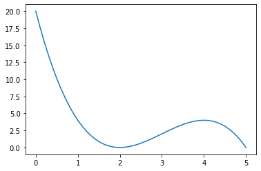
It is clear from the plot that there is a local minimum and a local maximum. We can verify the location of these points by differentiation:

\[\begin{align*} f^{\prime}(x)&=-3 x^2+18x-24 \\ &= -3(x-2)(x-4), \qquad f^{\prime}(x)=0 \implies x=2,4. \end{align*}\]

It is also possible to numerically obtain the location of the stationary points using the scipy optimization library, but the results obtained this way will not be exact. For example:

from scipy import optimize
xmin_local = optimize.fminbound(f, 1, 3) #search for min in [1,3]

#To find the maximum of f(x) we can find the minimum of g(x)=-f(x)
g = lambda x: -f(x)
xmax_local = optimize.fminbound(g, 3, 5) #search for min in [3,5]

print(xmin_local)
print(xmax_local)

2.0000014309459067
3.9999985690515034

7.6.1. Classification by hand

We can classify stationary points without the use of a plot by looking algebraically at the slope of the curve either side of each stationary point. This can be useful if we want to find general results that do not rely on producing a plot for each scenario.

It is convenient to record the results in a table, as demonstrated below for the function (7.10). We know that the gradient changes sign only at the points :x=2 and x=4, so we can conveniently choose the test points as follows.

	x=1	x=2	x=3	x=4	x=5
f^{\prime}(x)	-	0	+	0	-

From the table, we can infer that \(x=2\) is a local minimum and \(x=4\) is a local maximum.

Exercise 7.12

Can you guess the sign of the second derivative at the points \(x=2,4\) ?

The second derivative measures the rate of change of the slope \(s\), since

\[\begin{equation*} \frac{\mathrm{d}^2f}{\mathrm{d}x^2} =\frac{\mathrm{d}}{\mathrm{d}x}\frac{\mathrm{d}f}{\mathrm{d}x}=\frac{\mathrm{d}s}{\mathrm{d}x}, \end{equation*}\]

• When \(f^{\prime\prime}(x)>0\) the slope is increasing

• When \(f^{\prime\prime}(x)<0\) the slope is decreasing

Since the slope at \(x=2\) is going from negative to positive, the second derivative at this point will be positive (increasing).

Since the slope at \(x=4\) is going from positive to negative, the second derivative at this point will be negative (decreasing).

We can therefore use the second derivative to classify local maxima/minima. However, this test is not conclusive for the case when the second derivative is equal to zero.

In addition to maxima and minima we have the possibility of another type of stationary point called a point of inflection. This occurs when the slope of a function becomes zero without changing sign. The most basic example of an inflection point is for the function \(y=x^3\), which is stationary at \(x=0\). Plots of the function and its derivative are illustrated below:

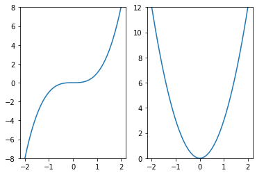
Fig. 7.2 [Left] \(y=x^3\), [Right] \(y=3x^2\).
The cubic has an inflection point at \(x=0.\)

Exercise 7.13

Show that the function \(f(x)=x^4-8x^3+24x^2-32x+23\) has a stationary point at \(x=2.\)

What does the result \(f^{\prime\prime}(2)\) tell you about this point? Is this point a local maximum/minimum/inflection?

\(f^{\prime}(x)=4x^3-24x^2+48x-32\)
\(\implies f^{\prime}(2)=32-96+96-32=0\)

\(f^{\prime\prime}(x)=12x^2-48x+48\)
\(\implies f^{\prime\prime}(2)=48-96+48=0\)

This result doesn’t tell us anything about the stationary point! It could be a local maximum/minimum or a point of inflection.

In this case the slope is increasing either side of the stationary point, so the point is a minimum:

\(f^{\prime\prime}(x)=12(x^2-4x+4)=12(x-2)^2 \geq 0 \ \forall x\)

Exercise 7.14

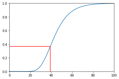
The Gompertz curve is given by

\[\begin{equation*} y = a e^{-be^{-ct}}, \qquad a,b,c>0. \end{equation*}\]

It can be used in various modelling scenarios, such to model population growth, spread of disease and growth of tumours.

Show that \(y^{\prime\prime}=0\) when \(t=\ln(b)/c\). What is the significance of this result?

Notice that \(y\) is strictly positive for all \(t\).

Differentiating once:

\[\begin{equation*} \frac{\mathrm{d}y}{\mathrm{d}t}=a e^{-be^{-ct}}\frac{\mathrm{d}}{\mathrm{d}t}\biggr[-be^{-ct}\biggr]=ybce^{-ct} \end{equation*}\]

The first derivative is strictly positive for all \(t\).

Differentiating again:

\[\begin{equation*} \frac{\mathrm{d}^2 y}{\mathrm{d}t^2}=bc\biggr[-cye^{-ct}+e^{-ct}\frac{\mathrm{d}y}{\mathrm{d}t}\biggr]=ybc^2e^{-ct}\biggr[be^{-ct}-1\biggr] \end{equation*}\]

The second derivative changes sign when

\[\begin{equation*} be^{-ct}=1 \quad \implies \quad t=\frac{\ln(b)}{c} \end{equation*}\]

This point is a (non-stationary) inflection. A plot of the curve is shown below

import numpy as np
import matplotlib.pyplot as plt

# example parameters
a=1;b=50;c=0.1

t=np.linspace(0,100)

# plot the function
pwr=-b*np.exp(-c*t)
y=a*np.exp(pwr)
plt.plot(t,y)

# inflection point
tinf=np.log(b)/c
yinf=a/np.exp(1)
plt.plot([tinf,tinf,0],[0,yinf,yinf],'r')

plt.xlim([0,100])
plt.ylim([0,1])
plt.show()

7.7. Manoeuvring a ladder

The figure below illustrates the problem of getting an object around a corner between two corridors. We will imagine that the object has extendable length so that at any angle of placement \(\theta\) it just touches the corner and the walls of each corridor.

By calculating the length for each angle we will be able to find the maximum length of object that will fit around the corner.

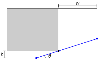
Fig. 7.3 Getting an object around a corner. The object is shown in blue, and the corridor widths have been denoted by \(h\) and \(w\). It is assumed here that the object is very thin, relative to the size of the corridors.

Exercise 7.15

Find an expression for the length of the line \(L\) in terms of \(\theta,h,w\), and plot \(L(\theta)\) for the case when \(h=1\), \(w=3\). Use your result for \(L(\theta)\) to find the longest object that will fit around the corner.

It is convenient to take the corner to be the origin of the coordinate system. The equation of the line through the point \((0,0)\) with gradient \(m\) is then given by

\[\begin{equation*} y=m x, \qquad m=\tan(\theta). \end{equation*}\]

The points where this line meets the boundary are

\[\begin{equation*} (-h/m,-h), \quad (w,mw) \qquad \implies \quad L=\sqrt{(w+h/m)^2+(mw+h)^2}. \end{equation*}\]

The minimum occurs when \(\frac{\mathrm{d}L}{\mathrm{d}m}=0\), but it is more convenient to differentiate the square of \(L\) :

\[\begin{align*} \frac{\mathrm{d}L^2}{\mathrm{d}m} = 0 \qquad &\implies \quad 2(w+h/m)(-h/m^2)+2(mw+h)w = 0\\ &\implies (mw+h)(w-h/m^3)=0 \quad \implies m=(h/w)^{1/3} \end{align*}\]

We can plot the length as a function of \(\theta\)

import numpy as np
import matplotlib.pyplot as plt

x = np.linspace(10,80,100) # in the range from [10,80] degrees
t = np.radians(x)          # convert to radians
m = np.tan(t)

w=3; h=1

def L(m):
  return np.sqrt((w+h/m)**2+(w*m+h)**2)

m0=(h/w)**(1/3)               #location of minimum
x0=np.degrees(np.arctan(m0))  #convert to angle

plt.plot(x,L(m))
plt.plot(x0,L(m0),'o')
plt.xlabel(r'$\theta$')

plt.show()


print([x0,L(m0)])

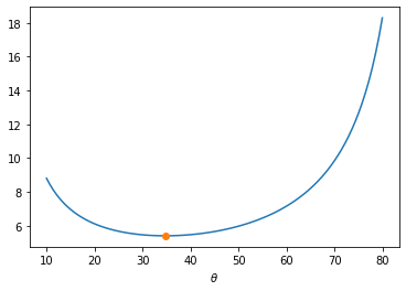
[34.735940696947736, 5.405598727423484]

The minimum occurs when \(\theta=34.73^{\circ}\). The longest object that can fit around the corner is 5.40 units. Here is an animation of the object being manoeuvred around the corner :