3. Exponential trends

Scale of student loans in England

The Government forecasts the value of outstanding loans to reach around £460 billion (2021-22 prices) by the mid2040s.

This chapter introduces the natural exponent and natural logarithm. After working through this chapter you should be able to:

• Calculate absolute and relative growth rates from a given dataset

• Understand the relationship between exponential behaviour and growth rates

• Manipulate exponentials and logarithms algebraically

3.1. Student debt in England

The table below shows how the amount of student debt in England has changed since 2005. Data are obtained from House of Commons Student Loan Statistics [page 35, table 2].

Table 3.1 Public student loan debt of English domiciled students and EU students studying in England (£ million)

2005	2006	2007	2008	2009	2010	2011	2012	2013
13033	15322	18116	21944	25963	30489	35186	40272	45903
2014	2015	2016	2017	2018	2019	2020	2021	2022
54355	64735	76253	89344	104457	121813	140093	160594	181612

Exercise 3.1

Calculate the yearly ratios of student loan debt, and hence calculate the average (mean) annual growth in student loan debt since 2005 as a percentage figure.

If the historic growth trend continues, in what year will student loan debt reach twice the figure that it is today?

Click to show

Code to calculate and print the results is given below. The yearly ratios are quite consistent, ranging from a minimum of 1.131 to a maximum of 1.211. The mean ratio is 1.168, and so the mean annual growth in student loan debt since 2005 is 16.8%.

import numpy as np
import pandas as pd

#Copy the data
x=np.arange(2005,2022,1)
y=np.array([13033, 15322, 18116, 21944, 25963, 30489, 35186, 40272, 45903,
  54355, 64735, 76253, 89344, 104457, 121813, 140093, 160594, 181612])

#Calculate the ratios
r=y[1:]/y[0:-1]

#Calculte the mean increase as a fraction
mu=np.mean(r)-1
print('Mean annual growth: {:<5.1%}'.format(mu))

#---------------------------------------------------------------------------
#The following lines are just to print the results in "pretty" format

dict={'year':x.astype('int'),'ratio':r}         #create data dictionary
df=pd.DataFrame(dict)                           #convert to dataframe (table)
df['ratio'] = df['ratio'].map('{:,.2f}'.format) #adjust format of ratio column
df

Inspecting the data in Table 3.1 we can see that the debt figure doubled roughly every five years. If the growth rate remains roughly constant (as it has over the last 17 years) we can expect that the student loan debt will reach twice its current value by 2027.

The five-year result can be related to the annual growth figure that we calculated. If we take the amount in a given year to be $D_0$ then the amount in the $n^{\text{th}}$ subsequent year should be given by the expression

$$D=D_0(1.168{)}^n.$$

Taking $n=4$ gives a result a bit less than $2D_0$, whilst taking $n=5$ gives a result a bit bigger than $2D_0$.

---

Exercise 3.2

Plot the student loan data $(t,D)$ given in Table 3.1 together with the curve defined by

$$D=D_0(1+r{)}^{t-t_0}$$

with $r=0.168$, $t_0=2005$, $D_0=13033$.

Click to show

import matplotlib.pyplot as plt

D0=13033; t0=2005; r=0.168

t=np.linspace(2005,2022,100)
D = D0*(1+r)**(t-t0)

plt.plot(x,y,'ok')

#prettify
plt.plot(t,D)
plt.xticks([2005,2010,2015,2020])
plt.xlabel('Year')
plt.ylabel('Student debt (£ million)')
plt.show()

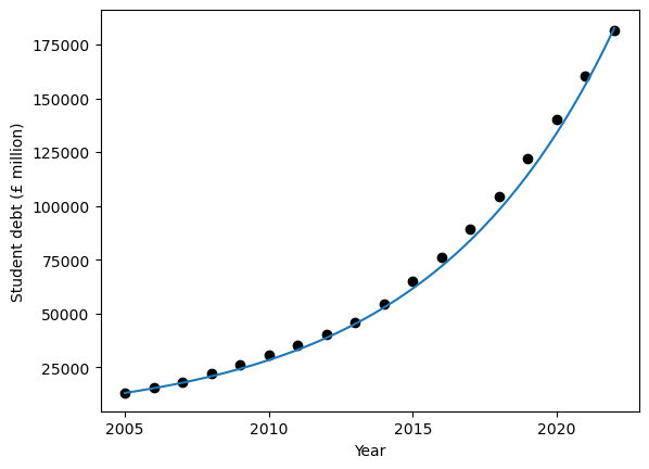
Notice that when plotting the curve we have evaluated the expression for $D$ not only at the whole-number values of $t$, but also in between. We have used a continuous function to represent discrete data.

---

Exercise 3.3

Using the function $D=D_0(1.168{)}^T$, where $T$ is measured in years, give estimates of the monthly, daily and hourly fractional growth. Convert your answers to fractional growth rates by dividing by the timescale.

Click to show

The fractional growth in an amount of time $T_{step}$ is given by the formula below:

$$\frac{D_{step}}{D}=\frac{D_0(1.168{)}^{T+T_{step}}-D_0(1.168{)}^T}{D_0(1.168{)}^T}=(1.168{)}^{T_{step}}-1.$$

To convert to a rate we divide the result by $T_{step}$

Timescale	$T_{step}$	growth fraction	growth rate
Monthly	$1/12$	$1.30\times {10}^{-2}$	$0.156302$
Daily	$1/365$	$4.26\times {10}^{-4}$	$0.155326$
Hourly	$1/8760$	$1.77\times {10}^{-7}$	$0.155294$

We can represent what we have done graphically:

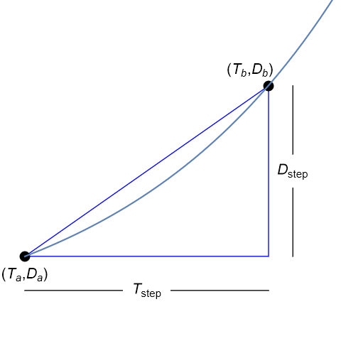
The slope of the line connecting points shown on the curve is

$$k=\frac{D_{step}}{T_{step}}=\frac{D_b-D_a}{T_b-T_a}$$

This value is the absolute growth rate. Dividing by the initial value $D_a$ gives the relative (fractional) growth rate.

3.2. Exponential relationships

An exponential relationship has the following form, where $y_0$ and $k$ are constants:

(3.1)$$y=y_0{k}^x.$$

In the previous section on student loans we saw an example with $k=1.168.$ The plot below shows how the exponential curve looks for some other values of $k$, taking $y_0=1$. By putting $x=0$ we obtain $y=y_0$, so this is the value at which the curve meets the vertical axis.

import numpy as np
import matplotlib.pyplot as plt

x=np.linspace(-4,4,100)

plt.plot(x,0.5**x,'k')
plt.plot(x,1.5**x,'r')
plt.plot(x,2.0**x,'b')
plt.show()

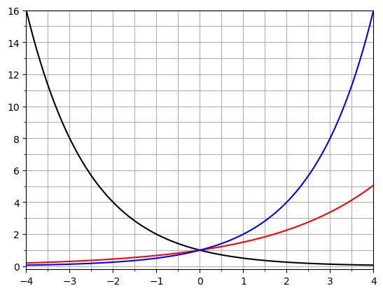
Fig. 3.1 Exponential function $y=k^x$ for $k=0.5$ [black], $k=1.5$ [red], $k=2.0$ [blue].

Notice that the plots for $k=0.5$ and $k=2.0$ are mirror images in the vertical axis. This can be understood from the laws of exponents:

(3.2)$$k^{-x}=(k^x{)}^{-1}=\frac{1}{k^x}={\left(\frac{1}{k}\right)}^x.$$

We can describe the shape of the exponential curve for values of the positive constant $k$ :

• For $k>1$ it starts off quite flat, but grows quickly as $x$ increases.

• For $k<1$ it first decreases quickly towards zero before a slow decline.

A more precise description is given by looking again at the growth rate. As discussed in Exercise 3.3, the absolute growth rate is given by

(3.3)$$\frac{y_{step}}{x_{step}}=\frac{k^x(k^{x_{step}}-1)}{x_{step}}=y\left(\frac{k^{x_{step}}-1}{x_{step}}\right)$$

The final value in brackets is the relative growth rate, which is constant for a particular value of $x_{step}$. Therefore the absolute growth rate for this function is proportional to $y$.

This is why we see exponential growth in problems where the rate of change in a quantity is proportional to the quantity itself. Examples include :

• compound interest, where the amount of interest is proportional to the cash amount

• population growth${}^{\ast }$, where the number of births is proportional to the population size.

${}^{\ast }$ This is only true to an extent. Populations typically do not grow exponentially over the medium-to-long term. See (for example) ourworldindata.org

The expression (3.3) depends on $x_{step}$, but we are interested in the instantaneous growth rate as $x_{step}$ approaches zero. Numerically we cannot take $x_{step}=0$ since “0/0” is indeterminate. However, we can try some small values.

Exercise 3.4

Calculate the relative growth rate for some values of $k$ with xstep=1e-10. For what value of $k$ is the relative growth rate equal to one? See of you can find this value to 3 decimal places.

Click to show

A plot can help us see the relative growth rate for different values of $k$ at a glance:

import numpy as np
import matplotlib.pyplot as plt


xstep = 1e-10

k = np.linspace(1,4,100)
r = (k**xstep - 1)/xstep

plt.plot(k,r)
plt.show()

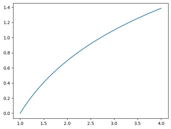
From the plot we can see that the value giving a relative growth rate of one is around $k=2.7$. Trying some different values of $k$ allows us to bracket the value to within the range $(2.7182,2.7183)$

k = np.array([2.7182, 2.7183])
r = (k**xstep - 1)/xstep
print(r)

[0.999969   1.00000674]

Therefore we can say that to 3dp, $k=2.718$.

3.3. The natural exponent

The natural exponent $e$ can be defined as the constant for which the relative growth rate of $e^x$ is equal to one. In the previous section you found this value to three decimal places. Its value can be obtained to higher precision in python by using the exp function from the numpy library:

import numpy as np
print(np.exp(1))

2.718281828459045

If you need the value of $e$ to even higher precision, this is possible with the mpmath library, but for almost all practical purposes the numpy library value has plenty of accuracy. Computations with more digits are slower to carry out due to the way that computer memory is allocated, and so we should only use higher accuracy when really necessary. Here are the first 1000 digits of $e$ :

import mpmath as m
m.mp.dps = 1000
print(m.mp.exp(1))

2.718281828459045235360287471352662497757247093699959574966967627724076630353547594571382178525166427427466391932003059921817413596629043572900334295260595630738132328627943490763233829880753195251019011573834187930702154089149934884167509244761460668082264800168477411853742345442437107539077744992069551702761838606261331384583000752044933826560297606737113200709328709127443747047230696977209310141692836819025515108657463772111252389784425056953696770785449969967946864454905987931636889230098793127736178215424999229576351482208269895193668033182528869398496465105820939239829488793320362509443117301238197068416140397019837679320683282376464804295311802328782509819455815301756717361332069811250996181881593041690351598888519345807273866738589422879228499892086805825749279610484198444363463244968487560233624827041978623209002160990235304369941849146314093431738143640546253152096183690888707016768396424378140592714563549061303107208510383750510115747704171898610687396965521267154688957035035

The natural exponent can be used to capture exponential relationships with relative growth rates that are not equal to one. Consider an expression of the following form, where $\lambda$ is a constant:

$$y=e^{\lambda x}.$$

The relative growth rate is given by

$$\begin{array}{rl}\frac{1}{y}\frac{y_{step}}{x_{step}}& =\frac{e^{\lambda x_{step}}-1}{x_{step}}\\ & =\lambda \frac{e^q-1}{q},q=\lambda x_{step}\end{array}$$

We want to evaluate this expression as $x_{step}$ approaches zero, which is the same as allowing $q$ to approach zero. Therefore, the relative growth rate of $e^{\lambda x}$ is found to be $\lambda$. This helps us to recognise why $e$ is the “natural” exponent.

We can also relate other exponential forms to the natural exponent. By way of example, the plot below shows a comparison between

$$y_1=e^{0.693x},y_2=2^x.$$

It can be seen that the two functions are very close over the range of values plotted. By adjusting the value of $\lambda$ in the expression $y=e^{\lambda x}$ it is possible to make the result identical to $2^x$. We will see how this can be done in the next section.

import numpy as np
import matplotlib.pyplot as plt

x=np.linspace(0,10,100)

y1=np.exp(0.693*x)
y2=2**x

fig, axs = plt.subplots(2,1)
axs[0].plot(x,y1,x,y2)
axs[1].plot(x,np.abs(y1-y2))

plt.show()

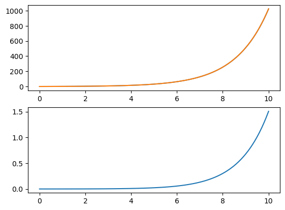
Fig. 3.2  Top :
 Bottom :  $y_1=e^{0.693x}$ and $y_2=2^x$ (overlapping)
$|y_2-y_1|$

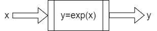
Notice that in python, we obtain $e^x$ by typing exp(x). It is helpful to think of exponentiation as a function, which takes an input value $x$ and returns an output value $y$ as illustrated in the schematic diagram below. A graph $(x,y)$ can depict the (input,output) relationship.

Exponentiation is not unique in this way: any mathematical (input,output) operation can be imagined as a function. For example, we might define the “squared” function that gives the area of a square with side-lengths $x$.

import numpy as np

y=np.square(3)
print(y)

9

Exercise 3.5

If you want to approximate the time it takes for an exponentially growing quantity to double, you can divide 70 by the percentage growth rate. For example, a population growing at 2% a year has a doubling time of about 35 years. Find an exact equation for the doubling time and explain why the rule of 70 works as an approximation.

Click to show

Let $T$ be the doubling time:

$$2=e^{\lambda T}\Rightarrow T=\frac{\ln (2)}{\lambda }$$

The quantity $\lambda$ is the growth rate given as a fraction.

If $\hat{\lambda }$ is the percentage growth rate then

$$T=\frac{100\ln (2)}{\hat{\lambda }}.$$

The value of 70 is a whole number approximation to $100\ln (2)$.

3.4. The natural logarithm

We now turn our interest to the inverse of the exponential function, which poses the following problem:

Given a certain value $y$, what value of $x$ satisfies the relationship $y=e^x$ ?

We will need to solve this problem to do algebra involving exponentials. Defining the exponential without its inverse would be like defining multiplication without division. In non-mathematical terms it would be like having the ability to put your shoes on but no way to take them off again!

Thinking about the (input,output) relationship of the exponential function, we can see that the (output,input) graph can be obtained by swapping the x and y axes. This is equivalent to a reflection in the line $y=x$, as shown in the figure below. This relationship with the inverse is true for all functions. For example, the graph of the square root function can be obtained by reflecting the squared function in the line $y=x$.

We call the inverse of the (natural) exponential function the natural logarithm, and we denote it by $\ln (x)$.

import numpy as np
import matplotlib.pyplot as plt

x=np.linspace(0,2,100)
y=np.exp(x)

plt.plot(x,y, label='$y=e^x$')
plt.plot(y,x, label='$y=\ln(x)$')
plt.plot([0,5],[0,5],'k') #y=x

#prettify
plt.grid()
plt.legend()
plt.show()

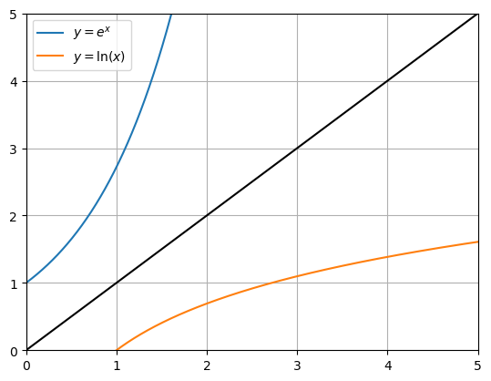
Fig. 3.3 The exponential function together with its inverse.

We can get an estimate of the natural logarithm by reading off from the graph. For instance, we can see that $e^x=2$ is obtained when $x$ is roughly equal to 0.7. We can obtain a more precise result by bracketing the value:

import numpy as np
print(np.exp([0.6931,0.6932]))

[1.99990564, 2.00010564]

The value lies between (0.6931,0.6932) so we can conclude that it is 0.693 to 3 decimal places. Its value can be obtained to higher precision in python by using the log function from the numpy library:

import numpy as np
np.log(2)

0.6931471805599453

The log function from the numpy library gives the natural logarithm. This can confuse some students who have previously encountered the logarithm in base 10. The logarithm in base 10 can be found using the log10 function from the numpy library. We will discuss different base logarithms in Section 3.6.

3.5. A tremendously useful result

Due to the way that we have defined the logarithm as the inverse of the exponential function we can say that the following two expressions are logically equivalent, as indicated by the symbol $⟺$, which can be read as “implies and implies that”:

(3.4)$$y=e^x⟺x=\ln (y)$$

We can also combine these equivalent statements into a single result, which highlights the way that inverse functions work:

(3.5)$$x=e^{\ln (x)}\text{ or }x=\ln (e^x).$$

In either of the two forms above, we see that applying one function followed by its inverse takes us back to where we started. In non-mathematical terms it’s like putting your shoes on and then taking them off again.

The result (3.5) can be used to make the following comparison:

$$k^x={\left(e^{\ln (k)}\right)}^x=e^{\ln (k)x}$$

The result on the RHS is of the form $e^{\lambda x}$ with $\lambda =\ln (k)$. We have learned that $k^x$ is equivalent to “natural” exponential growth with a relative growth rate factor $\lambda =\ln (k)$. This now explains the value $\ln (2)\simeq 0.693$ that was used to match the curves in Fig. 3.2.

3.6. All your base are belong to us

The natural logarithm is not the only logarithm that we can define. We could find the inverse of any expression of the form $k^x$. A commonly used example is the logarithm corresponding to $y={10}^x$, which we call the logarithm in base 10. It is often used because of our decimal number system, which uses powers of 10.

The logarithm in base 10 can also be related to the logarithm in base $e$:

$$y=\text{log10}(x)⟺{10}^y=x⟺{\left(e^{\ln (10)}\right)}^y=x⟺e^{y\ln (10)}=x.$$

Taking logarithm of both sides in the final expression:

$$y\ln (10)=\ln (x)⟺y=\frac{\ln (x)}{\ln (10)}.$$

Since we originally defined $y$ as the base 10 logarithm of $x$ we have the result

(3.6)$$\text{log10}(x)=\frac{\ln (x)}{\ln (10)}.$$

By using exactly the same algebra we can dwmonstrate that the analogous result applies to the logarithm in any base:

(3.7)$${\log }_k(x)=\frac{\ln (x)}{\ln (k)}.$$

We can also use the relationship between the exponential function and its inverse to derive the following three results, which apply in any base:

Laws of logarithms

The following useful results can be derived:

• $\log (ab)=\log (a)+\log (b)$

• $\log (x^n)=n\log (x)$

• $\log (a/b)=\log (a)-\log (b)$

3.7. Problems for you to try

[1] Write the expression $\log (32)-3\log (4)+\log (3)$ as a single logarithm

Click to show

$\log \left(\frac{32\times 3}{4^4}\right)=\log \left(\frac{3}{2}\right)$

[2] Find the value of $x$ for which ${\log }_2(x^2+4x+3)-{\log }_2(x^2+x)=4$

Click to show

${\log }_2\left(\frac{x^2+4x+3}{x^2+x}\right)=4$ gives $\frac{x^2+4x+3}{x^2+x}=2^4$.

This which rearranges to a quadratic with solutions $x=-1$, $x=1/5$.

The negative solution is not applicable. Why?

[3] Solve the problem $3^x=8$ by taking logarithms

Click to show

$x\log (3)=\log (8)$ gives $x=\frac{\log (8)}{\log (3)}=1.89$ (3sf)

[4] Calculate the result ${\log }_7(29)$ in terms of the natural logarithm

Click to show

${\log }_7(29)=\frac{\ln (20)}{\ln (7)}$ or we can solve this problem as follows:

Let $y={\log }_7(29)$. Then $7^y=29$.

Using $7=e^{\ln (7)}$ gives $y\ln (7)=29$ from which the result is immediately obtained.

[5] Solve the problem $\log (x)+\ln (x)=2$

Click to show

$\frac{\ln (x)}{\ln (10)}+\ln (x)=2$ gives $\ln (x)=\frac{2\ln (10)}{1+\ln (10)}$,

So $x=\exp \left(\frac{2\ln (10)}{1+\ln (10)}\right)=4.03$ (3sf)

[6] The hyperbolic cosine function is defined as $\cosh (x)=\frac{1}{2}(e^x+e^{-x})$. By rewriting the equation $\cosh (x)=4$ as a disguised quadratic in $e^x$, solve to find the two possible values of $x$. Give your answers as exact values involving the natural logarithm.

Click to show

The given problem is $\frac{1}{2}(e^x+e^{-x})=4$.

By taking $y=e^x$ we can write this as $y+\frac{1}{y}=8$.

This can be rearranged as $y^2-8y+1=0$ with solutions $y=4\pm \sqrt{15}$.

Since $y=e^x$ the solutions to the given problem are $x=\ln (4\pm \sqrt{15})$.