15. Peak oil

Energy Research and Social Science

In 2010, an in-depth review of over 500 studies concluded that the global peak in oil supply was likely to take place before 2030, and possibly even before 2020.

This case study is provided for you to explore the mathematics of the logistical model. You will be asked to critically evaluate the application of this model to the historic problem of determining when oil supplies may be insufficient to meet world demand.

15.1. Resource exploitation

The exploitation of a non-renewable resource cannot continue forever. If a supply \(S\) is extracted at constant rate \(C\) per year, then the resource will be fully exhausted in time \(t=S/C\).

Resource exploitation is typically not constant. Rates of extraction are often seen to increase over time (e.g. due to supplier-induced demand). The rate of exploitation may increase for as long as the resource is sufficiently abundant and available. However, as the resource becomes increasingly scarce or difficult to access the rate of exploitation is expected to decline. Peak production refers to the point in time at which exploitation of the resource is greater than at any time before or after.

These ideas can be developed into a mathematical model, and by fitting the model to available data we can attempt to make predictions about future supply of resources. In the 1950s and 60s such analyses led to predictions of an impending oil crisis. Into the early 2000s many authors were still using these models to confidently predict that world oil production would peak by the end of the first decade of the millennium.

15.2. Dataset

In this case study we will examine a mathematical model of resource-limited growth and apply it to oil production data from a single country. You will be asked to provide your thoughts on the model.

The dataset that we will use are found at ourworldindata.org. We will examine the dataset for oil usage in the United States only. After completing this case study, if you want to try out the mathematics for another country you are welcome to include your additional work in your submission.

The US dataset can be downloaded from us-oil.csv.

Exercise 15.1

Import and plot the dataset for US oil production. What trends do you observe?

15.3. The model

The logistic model applies to scenarios where we anticipate exponential growth that levels off due to resource restrictions. It has been utilised in a tremendous range of scientific and non-scientific applications.

The model is traditionally defined with reference to a population, but here we will instead refer to stock, which we will define as the total amount of resource produced over a period of time. We let \(x(t)\) be the stock at time \(t\). It is assumed that the environment has sufficient resource to support a maximum stock size \(C>0\), called the carrying capacity. Write down an expression for the fraction of remaining resource when the stock size is \(x\).

Fraction remaining: \(\displaystyle 1-\frac{x}{C}\).

Assume that the relative rate of change of stock is proportional to the fraction of available resources, with constant of proportionality \(r>0\). Write down a differential equation for \(x(t)\). This is the logistic model.

\[\begin{equation*} \frac{1}{x}\frac{\mathrm{d}x}{\mathrm{d}t}=r\left(1-\frac{x}{C}\right), \qquad x(0)=x_0. \end{equation*}\]

15.4. Numeric solution

Exercise 15.2

By using the discrete differentiation formula,

\[\begin{equation*} \frac{\Delta x}{\Delta t} = \frac{x_{i+1}-x_i}{t_{i+1}-t_i} \end{equation*}\]

with a common difference \(h=\Delta t\), write down an expression for \(x_{i+1}\) and hence obtain a numeric estimate of the curve \(x(t)\) for the case where \(r=1.5\), \(C=75\), \(x_0=1\)

15.5. Analytic solution

The logistic model is satisfied by

(15.1)\[\frac{x}{x-C}=\frac{x_0 e^{rt}}{x_0-C}\]

Exercise 15.3

Verify this claim by differentiating the implicit equation (15.1) with respect to \(t\).

Exercise 15.4

Rearrange (15.1) to find an explicit expression for \(x(t)\) and hence find the limiting value(s) as \(t\rightarrow\pm\infty\)

15.5.1. Growth rates

According to the logistic model, the rate of change of stock \(x\) is given by the following production function:

\[\begin{equation*} P(x)=rx\left(1-\frac{x}{C}\right). \end{equation*}\]

Exercise 15.5

Produce a plot of the production function for parameter values \(r,C\) of your choice. Describe how the growth rate changes in relation to the carrying capacity. Explain how the production curve demonstrates that the stock size cannot exceed the carrying capacity in the long run.

Exercise 15.6

Show analytically that peak production occurs at half carrying capacity, and show that the time to peak is given by

\[\begin{equation*} \tau=\frac{1}{r}\ln\left(\frac{C}{x_0}-1\right) \end{equation*}\]

Note

Note: If \(g\) is discrete growth rate (e.g. annual growth rate) then \(r=\ln(1+g)\) and so we have

\[\begin{equation*} \tau=\frac{\ln(C/x_0-1)}{\ln(1+g)} \end{equation*}\]

15.6. Estimation from data

According to the logistic model, the relative growth rate obeys a linearly decreasing trend:

\[\frac{1}{x}\frac{\mathrm{d}x}{\mathrm{d}t}=\frac{P(x)}{x} = r-\frac{r}{C}x\]

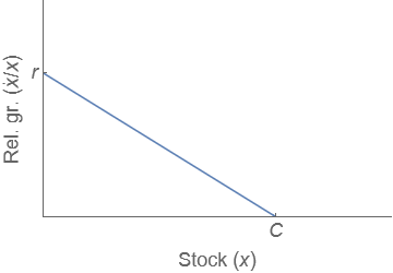
Fig. 15.1 Growth rate in logistic model

This provides a way to estimate the carrying capacity from a given dataset. We can numerically estimate the relative growth rate using a few initial points and then extrapolate to the axis. However, this can be dangerous. The pattern may not continue, or errors may be magnified.

Exercise 15.7

By using the US oil dataset for the years 1900 to 2008 only, estimate the carrying capacity \(C\) and the logistic production rate \(r\).

Hints:

• In this model, \(\Delta x/\Delta t\) is the amount of oil produced in a given year and \(x\) is the cumulative amount of oil produced.

• The relative growth rate estimate will not be accurate when \(x\) is small, as small fluctuations in data values have a large impact relative to the size of \(x\)

Due to data fluctuations, we should not expect that the datapoints will lie on the model curve, and therefore we should not expect that the first datapoint will give us a good choice of parameter \(x_0\).

Instead, we can use the following rearrangement of (15.1), which allows us to use the accumulated value for \(x\) up to the final datapoint - therefore making use of the whole dataset:

(15.2)\[\begin{equation} x_0 = \frac{C}{1+(C/x-1)e^{rt}} \end{equation}\]

Exercise 15.8

By using the parameter values \(r,C\) that you calculated, find an estimate for \(x_0\) and hence, plot the fitted approximation along with the US oil dataset. You should obtain a result that is somewhat similar to this one.

Exercise 15.9

With reference to your figure and to literature, write two or three paragraphs to explain whether you think the logistic model is useful to describe and/or predict world oil production in future.

You must write in your own words, and provide references to support your assertions where appropriate.