Rational functions
Contents
5. Rational functions#
What part of “inverse tangent function approaching an asymptote” did you not understand?
In this chapter we will look at functions of the form \(P(x)/Q(x)\), where \(P,Q\) are polynomials. The material will require us to use partial fractions and so an overview of that technique is provided as background material.
After completing the chapter you should be able to plot rational functions and identify any vertical, horizontal or oblique asymptotes.
5.1. Partial fractions#
Composing fractions means putting everything together over a common denominator. For example:
Decomposition is the reverse process (taking the fraction apart). We can get Python to do this for us by using the sympy library, as demonstrated for this example below:
from sympy import *
x = symbols('x')
y = (5*x+7)/(x**2+3*x+2)
apart(y)
Warning
Using from ... import * is dangerous, because some of the imported functions may overwrite the behaviour of default functions. However, as long as we are careful and as long as we only do this for one function library at a time, we should be ok.
Although we can get Python (or Wolfram Alpha) to do partial fraction decomposition for us, it may be helpful to understand a little about how it works.
5.1.1. Technique#
If the degree of the numerator \(m\) is greater than the degree of the denominator \(n\), we can split off a polynomial of degree \((m-n)\)
The remaining fraction can be decomposed so that the factors of the denominator each appear in a fraction by themselves
For each fraction in the decomposition the degree of the numerator should be less than the degree of the denominator
5.1.2. Examples#
\(\begin{alignat}{4} \mathbf{[1]}\quad &\frac{11x+3}{x^2+3x+2} && = \frac{A}{x+1}+\frac{B}{x+2}\\ \mathbf{[2]}\quad &\frac{2}{(x^2-1)(x+2)} && =\frac{Px+Q}{x^2-1}+\frac{C}{x+2}=\frac{A}{x+1}+\frac{B}{x-1}+\frac{C}{x+2}\\ \mathbf{[3]}\quad &\frac{x^3}{(x-1)^2} &&= Ax+B + \frac{Cx+D}{(x-1)^2} \end{alignat}\)
We can work out the unknown values \(A,B,C\dots\) by composing everything on the right:
\(\begin{alignat}{4} \mathbf{[1]}\quad &\frac{A}{x+1}+\frac{B}{x+2} && = \frac{A(x+2)+B(x+1)}{x^2+3x+2}\\ \mathbf{[2]}\quad &\frac{A}{x+1}+\frac{B}{x-1}+\frac{C}{x+2} && =\frac{A(x-1)(x+2)+B(x+1)(x+2)+C(x-1)(x+1)}{(x^2-1)(x+2)}\\ \mathbf{[3]}\quad &Ax+B + \frac{Cx+D}{(x-1)^2} &&= \frac{(Ax+B)(x-1)^2+(Cx+D)}{(x-1)^2} \end{alignat}\)
Comparing the numerators in the two sets of expressions we obtain
\(\begin{alignat}{4} \mathbf{[1]}\quad & 11x+3 && = A(x+2)+B(x+1)\\ \mathbf{[2]}\quad & 2 && =A(x-1)(x+2)+B(x+1)(x+2)+C(x-1)(x+1)\\ \mathbf{[3]}\quad & x^3 && = (Ax+B)(x-1)^2+(Cx+D) \end{alignat}\)
We choose the values of \(A,B,C\dots\) to obtain the correct multiple of each power of \(x\). A quick way to find the values in many cases is by substituting a value of \(x\) that makes some of the factors equal to zero. For instance, in expression [2],
putting \(x=-1\) gives \(A=-1\),
putting \(x=1\) gives \(B=1/3\),
putting \(x=-2\) gives \(C=2/3\).
Let’s check with Python:
apart(2/((x**2-1)*(x+2)))
We obtained the correct expression.
The technique of substituting \(x\) values doesn’t work as nicely in [3]. In this case it’s easiest to compare coefficients of each power of \(x\). Expanding out the numerator gives
For terms to match on the left and right hand sides we require \(A=1\), \(B=2\), \(C=3\), \(D=-2\). The fraction decomposition is therefore
This decomposition is correct, but it is not as far as we can go! Notice that we can write
The complete decomposition agrees with the result given by Python:
apart(x**3/(x-1)**2)
Exercise 5.1
Determine which of the following fractions can be further decomposed:
a. \(\displaystyle \frac{x}{x^2+1}\quad\)
b. \(\displaystyle\frac{1}{(x+1)^2}\quad\)
c. \(\displaystyle\frac{x}{(x+1)^2}\quad\)
d. \(\displaystyle\frac{x}{x^2-1}\quad\)
e. \(\displaystyle\frac{1}{x^2-1}\quad\)
f. \(\displaystyle\frac{x}{(x^2+1)^2}\quad\)
g. \(\displaystyle\frac{x^2}{(x^2+1)^2}\quad\)
h. \(\displaystyle\frac{x^3}{x^2-1}\)
They can all be further decomposed except (a,b,f):
(c) \(\displaystyle\frac{1}{1+x}-\frac{1}{(1+x)^2}\)
(d) \(\displaystyle\frac{1}{2(x-1)}+\frac{1}{2(x+1)}\)
(e) \(\displaystyle\frac{1}{2(x-1)}-\frac{1}{2(x+1)}\)
(g) \(\displaystyle\frac{1}{1+x^2}-\frac{1}{(1+x^2)^2}\)
(h) \(\displaystyle x+\frac{1}{2(x-1)}+\frac{1}{2(1+x)}\)
5.2. Plotting rational fractions#
A rational fraction is a quotient of two polynomials (a polynomial over polynomial). Expressions of this type appear very frequently in science and mathematics, since polynomials are often used to approximate the behaviour of other functions over a range of values. Being able to graph expressions of this type can help us to identify key features, which may be of interest.
We will start by taking a look at the following fraction:
The sympy library offers a quick way to construct a plot of the function, as shown in Fig. 5.1, from which we may notice the following features:
[1] The function appears to “jump” from a large positive value to a large negative value for a particular value of \(x\)
[2] The function appears to approximately follow a linear trend away from \(x=0\)
from sympy import *
x = symbols('x')
y = (3*x**2+2*x)/(1-2*x)
p1=plot(y,xlim=[-10,10],ylim=[-30,30])
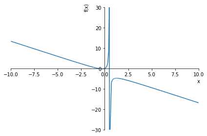
Fig. 5.1 Plotting the function \((3x^2+2x)/(1-2x)\) using sympy.#
We can understand the “jump” feature by looking at the denominator of the fraction (5.2), which has a root at \(x=1/2\). The function is undefined at this point. The graph below shows the behaviour of the numerator and denominator around \(x=1/2\).
import numpy as np
import matplotlib.pyplot as plt
x=np.linspace(-1,1,100)

fig,ax=plt.subplots()
plt.plot(x,3*x**2+2*x,label="numerator")
plt.plot(x,1-2*x,label="denominator")
plt.legend()
plt.xlim([-1,1])
plt.ylim([-1,5])
ax.axvline(0, color='k') # vertical axis
ax.axhline(0, color='k') # horizontal axis
plt.grid()
plt.show()
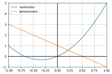
From the graph we see that:
As we approach \(x=1/2\) from the left by increasing \(x\), the denominator gets closer to zero whilst remaining positive.
As we approach \(x=1/2\) from the right by decreasing \(x\), the denominator gets closer to zero whilst remaining negative.
Meanwhile, the numerator approaches \(7/4\) in both cases. Thus, as the denominator shrinks in size the rational fraction “blows up”. The blow-up direction is positive or negative according to the sign of the denominator, which changes sign at \(x=1/2\).
The line connecting the positive and negative sections of the curve on the symbolic plot Fig. 5.1 is not a true feature of the function. It occurs because python produces a set of points and joins them up. In reality, the function is discontinuous at \(x=1/2\).
A more “proper” plot of the function is shown in Fig. 5.2. To produce the plot we force python to recognise the discontinuity by inserting nan (not-a-number) in the correct positions in the data series. The roots function from the numpy library can be used to find the roots of the denominator.
The line of values \(x=1/2\) is called a “vertical asymptote” of the function. Notice that the function value approaches the asymptote from either side.
import numpy as np
import matplotlib.pyplot as plt

[xmin,xmax]=[-10,10]
[ymin,ymax]=[-20,20]

x=np.linspace(xmin,xmax,1000)
y = (3*x**2+2*x)/(1-2*x)

xa = np.roots([-2,1])  #roots of 1-2x

# Set values to nan at discontinuity
loc=[np.argmax(x>i) for i in xa]
x=np.insert(x,loc,xa)
y=np.insert(y,loc,len(xa)*[np.nan])

plt.plot(x,y)

# Plot vertical asymptotes
for i in xa:
  plt.plot(2*[i],[ymin,ymax],'k--')

#Oblique asymptote
xx=np.array([xmin,xmax])
yy=-3/2*xx-7/4
plt.plot(xx,yy,'k--')

plt.xlim(xmin,xmax)
plt.ylim(ymin,ymax)
plt.show()
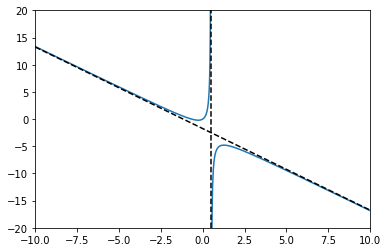
Fig. 5.2 Plotting the function \((3x^2+2x)/(1-2x)\) using numpy.#
To understand why the function follows a linear trend, we look at the partial fraction decomposition:
from sympy import *
x = symbols('x')
y = (3*x**2+2*x)/(1-2*x)
apart(y)
The decomposition allows us to analyse what happens to the function as \(x\) becomes large, in either the positive or negative direction. In that case, the value of \(1/(2x-1)\) becomes small, and so the function approaches the oblique asymptote
The sign of \(1/(2x-1)\) determines whether the function approaches the asymptote from above or below.
Exercise 5.2
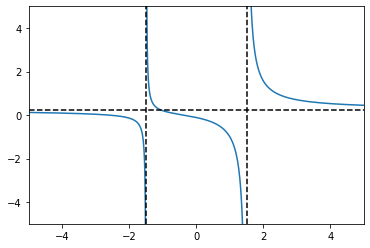
Produce a plot of the following function and identify any asymptotes:
It should be fairly easy to spot that the function has vertical asymptotes at \(x=\pm3/2\).
To find the other asymptotes, we can use partial fractions:
from sympy import *
x = symbols('x')
y = (x**2+3*x+1)/(4*x**2-9)
apart(y)
For large values of \(x\) the second and third terms in this decomposition shrink to zero and so the rational fraction approaches \(y=1/4\). This is a horizontal asymptote.
The plot is shown below
import numpy as np
import matplotlib.pyplot as plt

[xmin,xmax]=[-5,5]
[ymin,ymax]=[-5,5]

x=np.linspace(xmin,xmax,1000)
y = (x**2+3*x+1)/(4*x**2-9)

xa = np.roots([4,0,-9])  # roots of 4x^2-9

# Set values to nan at discontinuity
loc=[np.argmax(x>i) for i in xa]
x=np.insert(x,loc,xa)
y=np.insert(y,loc,len(xa)*[np.nan])

plt.plot(x,y)

# Plot vertical asymptotes
for i in xa:
  plt.plot(2*[i],[ymin,ymax],'k--')

#Other asymptote
xx=[xmin,xmax]
yy=2*[1/4]
plt.plot(xx,yy,'k--')

plt.xlim(xmin,xmax)
plt.ylim(ymin,ymax)
plt.show()