9. Simple models

The Language of Calculus, Strogatz

Without calculus, we wouldn’t have cell phones, computers, or microwave ovens. We wouldn’t have radio. Or television. Or ultrasound for expectant mothers, or GPS for lost travelers. We wouldn’t have split the atom, unraveled the human genome, or put astronauts on the moon. We might not even have the Declaration of Independence.

In this chapter we will start to write down some differential equations and “spot” their solutions. We will focus especially on the model for exponential growth. We will also begin to understand some other models by relating them to the exponential model for non-constant growth rate.

After working through the chapter you should be able to

• state the differential equation governing exponential growth/decay, and its corresponding solution for a particular initial condition.

• Examine models of non-constant growth via their relationship with the exponential model.

9.1. Describing change

Most things change, and we are already quite familiar with discussing how quickly they do so in our day-to-day lives. The formal study of time-dependent systems is called “mathematical dynamics”. To describe change we use the language of calculus because it allows us to write down mathematical models that govern the behaviour of systems. By investigating these models, we often can gain great insights about the systems they represent. It all starts with the first derivative, which defines the rate of change.

Note

We can also represent time derivatives using “dotty” notation in the following manner:

\[\begin{equation*} \dot{x}=\frac{\mathrm{d}x}{\mathrm{d}t}, \qquad \ddot{x}=\frac{\mathrm{d}^2x}{\mathrm{d}t^2} \end{equation*}\]

For a given quantity \(x\),

• if \(\mathrm{d}x/\mathrm{d}t>0\) then \(x\) is increasing

• if \(\mathrm{d}x/\mathrm{d}t<0\) then \(x\) is decreasing

In many scenarios the rate of change may depend on time \(t\) or on the value of \(S\) itself.

Exercise 9.1

Water flows out of a bucket at a constant rate of 0.1L/sec. Write down an equation for the amount of water \(V\) left in the bucket at time \(t\). Is it realistic?

Let \(V(t)\) be the amount of water (in litres) left in the bucket at time \(t\) (in seconds). According to the given information,

\[\begin{equation*} \frac{\mathrm{d}V}{\mathrm{d}t}=-0.1 \quad \Rightarrow V(t)=V_0 - 0.1t \end{equation*}\]

It works until the bucket is empty!

However, the rate of outflow may depend on water level in the bucket (e.g. due to pressure)

---

Exercise 9.2

Newton’s second law says that Force=mass \(\times\) acceleration.

Can you write this down as a problem involving velocity \(v\)?

We use the fact that acceleration is the rate of change of velocity to write result in mathematical form as:

\[\begin{equation*} F=m\frac{\mathrm{d}v}{\mathrm{d}t} \end{equation*}\]

We may also write the equation in terms of the displacement, using the fact that the velocity is the rate of change of displacement:

\[\begin{equation*} F= m \frac{\mathrm{d}}{\mathrm{d}t}\left(\frac{\mathrm{d}x}{\mathrm{d}t}\right)=m\frac{\mathrm{d}^2 x}{\mathrm{d}t^2} \end{equation*}\]

---

9.2. Exponential model

Before we write down the governing differential equation for exponential growth, let us first return to the case of discrete compound interest that we considered in the chapter on exponentials. We may describe this model using a difference equation involving discrete steps \(\Delta x\) and \(\Delta t\).

Exercise 9.3

A loan company charges interest of \(r\%\) per month. Write this down in the form of a difference equation. Also write down the general solution given an initial investment of \(x_0\)

In each time step \(\Delta t=1\)

\[\begin{equation*} \frac{\Delta x}{\Delta t} = \frac{\left(1+\frac{r}{100}\right)x-x}{1}=\frac{r}{100}x. \end{equation*}\]

The equation may be rearranged as

\[\begin{equation*} \frac{1}{x}\frac{\Delta x}{\Delta t} = \frac{r}{100}. \end{equation*}\]

The relative growth rate is constant, as we have seen previously for this model.

---

Exercise 9.4

Given a module of discrete compound growth of a quantity \(M\) with growth factor \(r\) and initial value \(M_0\), find the time to reach a given value.

\[\begin{align*} \frac{x}{x_0}=(1+r)^t \quad &\implies \quad \ln(x/x_0)=t\ln(1+r)\\ & \implies t=\frac{\ln(x/x_0)}{\ln(1+r)} \end{align*}\]

---

9.2.1. The continuous model

If interest is compounded continuously then it is convenient to write

\[\begin{equation*} x=x_0 e^{\lambda t}. \end{equation*}\]

We can relate this result to the discrete model by taking \(\lambda =\ln\left(1+\frac{r}{100}\right)\).

Differentiating then gives the model for exponential growth:

(9.1)\[\frac{1}{x}\frac{\mathrm{d}x}{\mathrm{d}t}=\lambda\]

According to the model, the relative growth rate is constant. In the case where \(x\) represents a population we can interpret this as the “per-capita” growth rate.

We could also express the equation in relation to the doubling time \(\tau\). For \(x\) to be doubled, \(x/x_0=2\) which gives

\[\begin{equation*} e^{\mu\tau}=2 \quad \Rightarrow \quad x=x_0 2^{t/\tau}\ . \end{equation*}\]

Exercise 9.5

Cocaine has a half-life of around 0.7-1.5 hour in human blood. Determine what percentage will remain after six hours.

Let \(\tau\) be the half-life. Then, when \(t=6\)hrs,

\[\begin{equation*} \frac{x}{x_0}=2^{-t/\tau} = \frac{1}{2^{6/\tau}} = [0.26 - 6.25]\%. \end{equation*}\]

You may wish to compare this to the results for caffeine and alcohol, which each have a mean half-life of about 5 hours.

---

9.3. Offset model

Exercise 9.6

In an offset exponential model, the rate of change of a quantity \(Q\) is proportional to the difference from some equilibrium value \(Q_e\) in the manner

\[\begin{equation*} \frac{\mathrm{d}Q}{\mathrm{d}t}=r(Q_e-Q) \end{equation*}\]

By defining \(D=(Q_e-Q)\), write down an equation for \(\dot{D}\) and solve it.

What do we mean when we say that \(Q_e\) is the equilibrium value?

Let \(D=(Q_e-Q)\), then

\[\begin{equation*} \frac{\mathrm{d}D}{\mathrm{d}t}=-rD \quad \rightarrow \quad \rightarrow D=D_0 e^{-r t} \end{equation*}\]

The equilibrium value is the point where \(\dot{Q}=0\). If the system reaches its equilibrium then it will remain there unless some external influence acts on the system to move it away from its equilibrium.

Notice that if \(r>0\) then

• when \(Q\) exceeds the equilibrium value the growth rate will be negative

• When \(Q\) is less than the equilibrium value the growth rate will be positive

Therefore this system wants to go to the equilibrium value.

Exercise 9.7

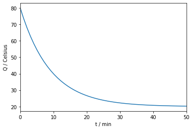
Apply the offset equilibrium model to find the time taken for a drink to cool from 80C to 63C given an ambient (room) temperature of 20C, given that \(r=0.11\)/min.

\[\begin{equation*} \ln(D/D_0)=-rt \quad \implies \quad t=\frac{-1}{0.11}\ln\left(\frac{20-63}{20-80}\right)=\frac{-1}{0.11}\ln(43/60) \end{equation*}\]

The drink will take 3 mins and 2 sec to reach the desired temperature.

Note that according to this model, the drink will never actually reach room temperature, though it will approach it in the limit.

A plot of this curve is shown below:

import numpy as np
import matplotlib.pyplot as plt

# example parameters
Qe=20; r=0.11; Q0=80;

t=np.linspace(0,50)
Q= Qe+(Q0-Qe)*np.exp(-r*t)

# plot the function

plt.plot(t,Q)
plt.xlim([0,50])
plt.xlabel('t / min')
plt.ylabel('Q / Celsius')
plt.show()

9.4. Microbial growth

The growth rate of a microorganism on a substrate demonstrates an S-shaped curve consisting of a “lag” phase (flat) followed by exponential growth, followed by a “stationary” (flat) phase.

To estimate the relative growth rate during the exponential phase we can fit a straight line to the logged data, as illustrated in the plot below. A worked exercise can be found in example 3.3 from the recommended reading on microbial growth.

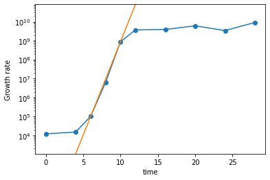
Fig. 9.1 After taking the logarithm we can identify the exponentially growing phase and find the constant growth rate.

The Monod equation is an empirical relationship that can be used to model the entire growth curve mathematically by taking into account the effect of substrate concentration on growth. It has the same form as the equation for molecular binding model that we looked at in Section 2.4. According to the model the specific growth rate \(\mu\) is given by

(9.2)\[\mu=\frac{\mu_{max}S}{K_s+S}\]

where \(\mu_{max}\) is the maximum growth rate, \(S\) is the substrate concentration, \(K_s\) is the half-saturation constant.

Exercise 9.8

Find leading order asymptotically equivalent expressions based on the Monod equation for :

• high substrate concentrations (\(S\gg K_s\))

• low substrate concentrations (\(S\ll K_s\))

At high substrate concentrations (e.g initially) the growth rate is approximately independent of the substrate concentration:

\(\qquad \displaystyle S\gg K_s\), so \(\mu = \mu_{max}\frac{1}{1+K_s/S}\sim \mu_{max}\).

At low substrate concentrations (late in evolution) the growth rate is proportional to the substrate concentration:

\(\qquad \displaystyle S\ll K_s\), so \(\mu=\frac{\mu_{max}S}{K_s}\left(1+\frac{S}{K_s}\right)^{-1}=\frac{\mu_{max}S}{K_s}\left(1-\frac{S}{K_s}+\dots\right)\sim \frac{\mu_{max}S}{K_s}\).

These features are what led Jacques Monod to propose model that uses his name.

---

Taking \(X\) to be the cell mass at time \(t\), we define the cell yield as the rate of cell mass production per unit of substrate consumed:

(9.3)\[Y=-\frac{\mathrm{d}X}{\mathrm{d}S} = \frac{\dot{X}}{-\dot{S}}\]

It is a constant, which depends on the substrate structure and the micro-organism. You may verify by differentiation that this equation is satisfied by

(9.4)\[S=S_0-\frac{1}{Y}(X-X_0)\]

where \(S_0\), \(X_0\) are the substrate concentration and cell mass when \(t=0\).

First notice that \((S_0,X_0)\) satisfies the equation. Then simply differentiation with respect to \(t\), treating \(Y\) as a constant:

\[\begin{equation*} \dot{S} = -\frac{1}{Y}\dot{X} \quad \implies Y=\frac{\dot{X}}{-\dot{S}} \end{equation*}\]

---

Putting (9.4) for the substrate concentration together with Monod’s growth rate gives

(9.5)\[\frac{\mathrm{d}X}{\mathrm{d}t} = \left[\frac{\mu_{max}S}{K_S+S}\right]X, \qquad S=S_0-\frac{1}{Y}(X-X_0).\]

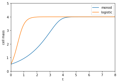
9.4.1. Monod vs logistic

Monod’s model may be compared to the logistic model, which is given by

\[\begin{equation*} \frac{\mathrm{d}X}{\mathrm{d}t}=rX\left(1-\frac{X}{C}\right) \end{equation*}\]

A comparison of the two model predictions for the cell mass is shown below. In the logistic model \(C\) denotes the “carrying capacity”, which is the maximum value of \(S\) that can be obtained. It occurs when the substrate is exhausted, \(S=0\), which gives

\[\begin{equation*} C=X_0+S_0 Y \end{equation*}\]

Taking \(r=\mu K/S_0\) ensures that growth rate in the logistic equation is equal to the growth rate in the Monod equation for low substrate concentrations.

Note

The exponential model is a special case of the logistic model with infinite carrying capacity.

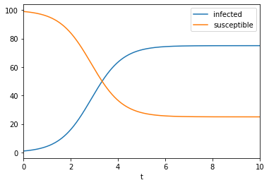
9.5. Flu transmission

A basic model of flu transmission is given below, in which \(S\) denotes susceptible individuals and \(I\) denotes infected individuals. The constants \(k\) and \(m\) in these equations are taken to be positive:

\[\begin{equation*} \begin{aligned} \frac{\mathrm{d}S}{\mathrm{d}t} &=-k SI+m I&& \text{[Equation I]} \\[10pt] \frac{\mathrm{d}I}{\mathrm{d}t} &=\phantom{-}k SI-mI && \text{[Equation II]} \end{aligned} \end{equation*}\]

Exercise 9.9

Give a physical interpretation of each term on the right hand side of the equation for \(\frac{\mathrm{d}I}{\mathrm{d}t}\).

\(kSI\) : When a susceptible person encounters an infected person this may result in infection. Infections occur at rate \(k\)

\(-mI\) : Infected individuals recover at rate \(m\)

Exercise 9.10

Taking \(N=(S+I)\), Find \(\frac{\mathrm{d}N}{\mathrm{d}t}\) and explain the result in terms of the population dynamics.

\(N=S+I\implies \frac{\mathrm{d}N}{\mathrm{d}t}=\frac{\mathrm{d}S}{\mathrm{d}t}+\frac{\mathrm{d}I}{\mathrm{d}t}=(-kSI+mI)+(kSI-mI)=0\)

This is a two compartment model. The total number of people in the population is constant.

Exercise 9.11

Use the result from Exercise 9.10 to write Equation II in the form

\[\begin{equation*} \frac{\mathrm{d}I}{\mathrm{d}t}= rI\left(1-\frac{I}{C}\right) \end{equation*}\]

where \(r,C\) are constants related to \(k,m,N\). Hence, write down the solution for \(I(t)\).

Taking \(N=100,k=0.02,m=0.5\), plot the solutions for \(I(t),S(t)\) on the same axes.

Substituting \(S=(N-I)\) into Equation II gives

\[\begin{equation*} \frac{\mathrm{d}I}{\mathrm{d}t}=rI\left(1-\frac{I}{C}\right) \end{equation*}\]

where \(r=(kN-m)\) and \(C=r/k\). Hence, the general form of the solution is given by

\[\begin{equation*} I= \frac{C}{1+(C/I_0-1)e^{-r t}}. \end{equation*}\]

import numpy as np
import matplotlib.pyplot as plt

# define parameters
N=100; k=0.02; m=0.5
r=k*N-m; C=r/k

# range to plot
t=np.linspace(0,10,1000)

# If there is initially one infection
I0=1

den = 1+(C/I0-1)*np.exp(-r*t)

I=C/den
S=N-I

plt.plot(t,I,label='infected')
plt.plot(t,S,label='susceptible')
plt.xlabel('t')
plt.legend()
plt.xlim([0,10])
plt.show()