8. Infinite powers

Siphonaptera

Great fleas have little fleas upon their backs to bite ‘em,

And little fleas have lesser fleas, and so ad infinitum

In the section on Asymptotic equivalence we saw some examples of polynomial approximations for common functions, such as \(f(x)=e^x\). We now outline the theory behind the results that were presented. After completing this chapter you should be able to:

• find Maclaurin and Taylor series expansions for given functions

• Discuss the convergence properties of these series using numeric justification

8.1. Motivation

We suppose that for “small” \(x\) we can express a given function \(f(x)\) as a sum of the form

(8.1)\[p(x) = c_0 + c_1x +c_2 x^2 + \dots + c_n x^n+\mathcal{O}(x^{n+1}).\]

The coefficients \(c_{0\dots n}\) will be chosen to give an accurate representation of \(f(x)\) in the neighbourhood of \(x=0\).

Exercise 8.1

Find the first three derivatives of \(p(x)\) and evaluate them at \(x=0\).

\(\begin{alignat}{10} p^{\prime}(x) &=c_1 &\ +\ & 2c_2x &\ +\ &3c_3x^2 &+\dots &+n c_n x^{n-1} &&+\mathcal{O}(x^n)\\ p^{\prime\prime}(x) &= &&2c_2 &\ +\ &6c_3x &+\dots &+n(n-1) c_n x^{n-2} &&+\mathcal{O}(x^{n-1})\\ p^{\prime\prime\prime}(x)&= && &\ \ & 6c_3 &+\dots &+n(n-1)(n-2) c_n x^{n-3} &&+\mathcal{O}(x^{n-2}) \end{alignat}\)

\(p(0)=c_0, \quad p^{\prime}(0)=c_1, \quad p^{\prime\prime}(0)=2c_2, \quad p^{\prime\prime\prime}(0)=6c_3\)

---

Exercise 8.2

Determine a general result for the \(n\)th derivative \(p^{(n)}(0)\).

Match this to \(f^{(n)}(0)\) to find an expression for \(c_n\).

\(p^{(n)}(x)=n!c_n+\mathcal{O}(x)\quad \implies p^{(n)}(0)=n!c_n\)

Assuming this matches \(f^{(n)}(0)\) gives \(c_n=\frac{f^{(n)}(0)}{n!}\)

Note: \(n!=n(n-1)(n-2)\dots 1\)
(e.g. \(6!=3\times 2=6\))

---

Exercise 8.3

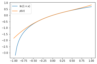
Calculate the first three non-zero terms in the expansion for \(f(x)=\ln(1+x)\), using the formula for the coefficients found in the previous exercise.

\(n\)	\(f^{(n)}(x)\)	\(f^{(n)}(0)\)	\(c_n\)
\(0\)	\(\ln(1+x)\)	\(0\)	\(0/0! = 0\)
\(1\)	\((1+x)^{-1}\)	\(1\)	\(1/1! = 1\)
\(2\)	\(-(1+x)^{-2}\)	\(-1\)	\(-1/2! = 1/2\)
\(3\)	\(2(1+x)^{-3}\)	\(2\)	\(2/3! = 1/3\)

The expansion is

\[\begin{equation*} p(x) = x-\frac{x^2}{2}+\frac{x^3}{3}+\mathcal{O}(x^4) \end{equation*}\]

We can plot this together with \(\ln(1+x)\) on the range [-1,1]. The representation is faithful close to \(x=0\), but gets worse away from this point, particularly in the negative \(x\)-direction.

import numpy as np
import matplotlib.pyplot as plt

x=np.linspace(-1,1)
y=np.log(1+x)

plt.plot(x,y,label=r'$\ln(1+x)$')
p=x-x**2/2+x**3/3
plt.plot(x,p,label='$p(x)$')
plt.legend()
plt.show()

---

Notice that if \(x\ll 1\) (“much less than one”) the higher powers are successively smaller. For instance, if \(x=0.1\) the \(x^3=0.001\). Therefore the leading terms are most significant in the expansion and the higher powers are “corrections”.

By way of example, consider the plots below, which show the curve \(y=e^x\) together with its linear, quadratic and cubic asymptotic expansions.

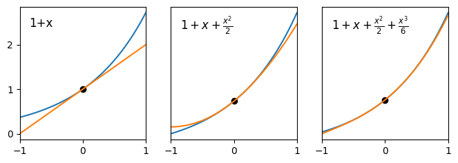
Fig. 8.1 Comparison of asymptotic expansions to the curve \(y=e^x\) on the domain \([-1,1]\).

We see that the linear approximation is an accurate representation of the curve in a very small domain close to \(x=0\), and that by adding the quadratic and cubic terms we successively improve the approximation on the domain \([-1,1]\).

8.2. Convergence

In the above discussion we have assumed that \(|x|<1\) so that the powers of \(x\) grow successively smaller. However, it is not guaranteed that the infinite sum \(p(x)\) will converge to \(f(x)\) on the whole interval \([-1,1]\). By constructing the expansion to match the derivatives of \(f(x)\) at \(x=0\) we have only ensured that the representation is accurate in some local neighbourhood of this point.

It is possible to use tools of mathematical analysis to formally determine the interval of convergence for the infinite series, which will be different for each function \(f(x)\). In the case of the series for \(\ln(1+x)\) it turns out that the infinite series converges to the correct value on the whole interval \([-1,1]\), albeit rather slowly for some values of \(x\).

What is truly remarkable is that for some functions the expansions constructed by the method outlined above are valid over a wider interval than \([-1,1]\). In fact, the expansions for some functions are valid for all values of \(x\). Examples include the functions \(e^x\), \(\sin(x)\) and \(\cos(x)\).

It is quite exciting to think that these non-polynomial functions can be represented by infinite polynomial series. However, the expansions converge increasingly slowly as we move further from the point \(x=0\), which lessens their practical use.

In this module we will not develop the tools of analysis required to undertake a formal investigation of convergence. We will adopt a more experimental approach, by generating series containing a few terms and evaluating their accuracy on the interval that we are interested in.

Exercise 8.4

Demonstrate that with only five terms in the expansion of \(\ln(1+x)\) we obtain a result that is accurate to within 1% on the interval \([-0.5,0.5]\)

import numpy as np
x=np.linspace(-0.5,0.5,1000)
y=np.log(1+x)

p=x-x**2/2+x**3/3-x**4/4+x**5/5

#maximum relative error
m=max(np.abs((y-p)/y))

#percentage error
print(100*m)

0.6644352054578373

The maximum relative error is 0.664%

---

Here is an example code to determine how many terms are required in the expansion to achieve a result within 1% of the numerically correct value on the interval \([-0.99,0.99]\). The code uses the following recursive formula for the terms \(u_n\) in the series for this function:

\[\begin{equation*} u_{n+1}=\left(\frac{-n x}{n+1}\right)u_n . \end{equation*}\]

import numpy as np
x=np.linspace(-0.99,0.99,1000)
y=np.log(1+x)

u=x    #nth term in series when n=1
p=x    #sum of first n terms

n=1
m=1   #to use in stopping condition

while m>0.01:
  u=-u*x*n/(n+1)         #next term in expansion
  p=p+u                  #add to running total
  m=max(np.abs((y-p)/y)) #maximum relative error
  n=n+1

print('n=%d' % n)

plt.plot(x,p)
plt.show()

Running this code tells us that 203 terms are required to obtain convergence to within 1%. Obviously that’s a lot of terms! For practical purposes, we normally want to use expansions with only a few terms.

8.3. Generalization

In the outline above we developed a power series expansion technique that was accurate in the neighbourhood of \(x=0\). For some series derived in this way the series can converge to the correct value on an extended interval. However, even where this is the case we normally require a large number of terms to be kept in order to obtain a good approximation away from the origin.

Where we require a power series approximation to a function near to a location other than \(x=0\), a better technique is to construct the expansion so that it has greatest accuracy in the neighbourhood of that point. We do this using a shifted version of the expansion formula:

(8.2)\[p(x;a)= c_0 +c_1(x-a)+c_2(x-a)^2+\dots +c_n(x-a)^n+\mathcal{O}\left((x-a)^{n+1}\right)\]

By applying the technique of matching derivatives at the location \(x=a\), we obtain the result

(8.3)\[c_n = \frac{f^{(n)}(a)}{n!}.\]

The formula (8.2) together with (8.3) is known as Taylor’s series. The special case when \(a=0\) is known as the Maclaurin series for historical reasons.

Exercise 8.5

Find the first four non-zero terms of the Taylor series for the following cases:

• \(e^{x}\) about the point \(x=1\)

• \(\sin(x)\) about the point \(x=\pi/3\)

\(n\)	\(f^{(n)}(x)\)	\(f^{(n)}(1)\)	\(c_n\)
\(0\)	\(e^x\)	\(e\)	\(e/0! = e\)
\(1\)	\(e^x\)	\(e\)	\(e/1! = e\)
\(2\)	\(e^x\)	\(e\)	\(e/2! = e/2\)
\(3\)	\(e^x\)	\(e\)	\(e/3! = e/6\)

Hence \(p(x;e)\sim e(1+x+x^2/2+x^3/6+\dots)\)

The result could have been obtained by recognising that

\[\begin{equation*} e^{1+x}=e^1 e^x \end{equation*}\]

and obtaining the expansion for \(e^x\) about \(x=0\).

\(n\)	\(f^{(n)}(x)\)	\(f^{(n)}(\pi/3)\)	\(c_n\)
\(0\)	\(\sin(x)\)	\(\sqrt{3}/2\)	\(\sqrt{3}/2/0! = \sqrt{3}/2\)
\(1\)	\(\cos(x)\)	\(1/2\)	\(1/2/1! = 1/2\)
\(2\)	\(-\sin(x)\)	\(-\sqrt{3}/2\)	\(-\sqrt{3}/2/2! = \sqrt{3}/4\)
\(3\)	\(-\cos(x)\)	\(-1/2\)	\(-1/2/3! = -1/12\)

Hence

\[\begin{equation*} p\left(x;\frac{\pi}{3}\right)\sim \frac{\sqrt{3}}{2}+\frac{x}{2}-\frac{\sqrt{3}}{4}x^2-\frac{x^3}{12} \end{equation*}\]

Exercise 8.6

Explain why it is not possible to construct a series expansion of \(\ln(x)\) about the point \(x=0\).

Also explain the relationship between the series for \(\ln(1+x)\) about \(x=0\) and the series for \(\ln(x)\) about \(x=1\).

The function \(\ln(x)\) is not defined at \(x=0\).

The series for \(\ln(x)\) about \(x=1\) is identical to the series for \(\ln(1+x)\) about \(x=0\).

This can be seen by defining \(\hat{x}=x-1\).

Exercise 8.7

A function \(W(x)\) is defined by the relationship

\[\begin{equation*} We^W =x. \end{equation*}\]

Although \(W\) cannot be expressed in terms of elementary functions, much is known about its properties. It is encountered in many areas of scientific study including neuroimaging, biochemistry, materials science, chemical engineering and quantum mechanics.

Show that \(\frac{\mathrm{d}W}{\mathrm{d}x}\) satisfies the result below and find an expression for \(\frac{\mathrm{d}^2 W}{\mathrm{d}x^2}\), giving your answer fully in terms of \(W\):

\[\begin{equation*} \frac{\mathrm{d}W}{\mathrm{d}x}=\frac{1}{e^W(1+W)}. \end{equation*}\]

Hence, find the Maclaurin series expansion of \(W\), up to and including the term in \(x^2\).

\[\begin{align*} We^W = x & \implies \frac{\mathrm{d}}{\mathrm{d}x}(W e^W)=1\\ & \implies \frac{\mathrm{d}W}{\mathrm{d}x}\left[e^W+We^W\right]=1\\ &\implies \frac{\mathrm{d}W}{\mathrm{d}x} = \frac{1}{e^W(1+W)} \end{align*}\]

Differentiating the result with respect to \(x\) gives:

\[\begin{align*} \frac{\mathrm{d}^2W}{\mathrm{d}x^2}&=\frac{\mathrm{d}W}{\mathrm{d}x}\frac{\mathrm{d}}{\mathrm{d}W}\left[\frac{1}{e^W(1+W)}\right]\\ & =\frac{1}{e^W(1+W)}\left[\frac{-\frac{\mathrm{d}}{\mathrm{d}W}[e^W(1+W)]}{e^{2W}(1+W)^2}\right]\\ &=\frac{-1}{e^W(1+W)^3}\frac{e^W(1+W)+e^W}{e^2W}=-\frac{(2+W)}{e^{2W}(1++W)^3} \end{align*}\]

Hence, the two term Maclaurin series expansion is

\[\begin{equation*} W(x)=x-x^2+\dots \end{equation*}\]

8.4. Midpoint rule

We argued in a previous chapter that the straight line connecting two data points ought to give a more accurate estimate of the slope at the mid-point of the interval, rather than at the left-hand point. The graphic below provides a characteristic justification of this claim:

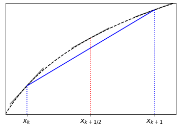
Fig. 8.2 The slope of the line connecting two points on a curve generally estimates the slope of the curve better at the midpoint of the interval than at the ends.

We may write:

\[\begin{equation*} s_{k+1/2} = \frac{y_{k+1}-y_k}{x_{k+1}-x_k} \end{equation*}\]

A proof of this result can be given using Taylor’s expansion.

Left-hand result

\[\begin{equation*} y(x+h) =y(x) +h y^{\prime}(x)+\mathcal{O}(h^2) \end{equation*}\]

Hence,

\[\begin{equation*} y^{\prime}(x) = \frac{y(x+h)-y(x)}{h} + \mathcal{O}(h) \end{equation*}\]

The error in this expression is proportional to \(h\).

---

Midpoint result

Taking the midpoint as \(\hat{x}=x+h/2\)

\[\begin{align*} y\left(\hat{x}+\frac{h}{2}\right)&=y(\hat{x})+\frac{h}{2}y^{\prime}(\hat{x})+\left(\frac{h}{2}\right)^2y^{\prime\prime}(\hat{x})+\mathcal{O}(h^3)\\ y\left(\hat{x}-\frac{h}{2}\right)&=y(\hat{x})-\frac{h}{2}y^{\prime}(\hat{x})+\left(\frac{h}{2}\right)^2y^{\prime\prime}(\hat{x})-\mathcal{O}(h^3) \end{align*}\]

Subtracting the second expression from the first gives

\[\begin{equation*} y\left(\hat{x}+\frac{h}{2}\right)-y\left(\hat{x}-\frac{h}{2}\right) = hy^{\prime}(\hat{x})+\mathcal{O}(h^3) \end{equation*}\]

Rearranging gives,

\[\begin{equation*} y^{\prime}(\hat{x}) = \frac{y(x+h)-y(x)}{h}+\mathcal{O}(h^2) \end{equation*}\]

The error in this expression is proportional to \(h^2\).

---

A comparison of the errors in the forward and central difference formulae is given below for the example of differentiating the function

\[\begin{equation*} y=\sin(x)+x. \end{equation*}\]

The code uses the fdiff function that was defined in the previous chapter.

# data points
x=np.linspace(-np.pi,np.pi,100)
y = np.sin(x)+x

# derivative estimate
yd=fdiff(x,y)

# analytic expression for derivative
def yp(x):
  return np.cos(x)+1

fig,ax = plt.subplots(2,1, figsize=(8, 8))

xlhs=x[0:-1]                    #left-hand x values
err = yd-yp(xlhs)               #error using forward estimate
ax[0].plot(xlhs,np.abs(err))    #plot size of error

xctr=(x[0:-1]+x[1:])/2          #midpoint x values
err = yd-yp(xctr)               #error using midpoint estimate
ax[1].plot(xctr,np.abs(err))    #plot size of error

plt.show()

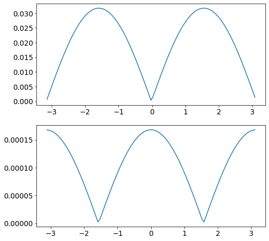
Fig. 8.3 Errors in the numeric derivative of \(y=\sin(x)+x\) on \([-\pi,\pi]\) with 100 datapoints.
\(\qquad \)(top) forward difference, (bottom) midpoint rule.

Note

Although the central difference formula is more accurate when the step size is large, both expressions become exact in the limit \(h\rightarrow 0\). The forward derivative formula is easier to work with.