Know your limits
Contents
6. Know your limits#
Bishop George Berkeley (1685-1753)
And what are these Fluxions? The Velocities of evanescent Increments? And what are these same evanescent Increments? They are neither finite Quantities nor Quantities infinitely small, nor yet nothing. May we not call them the ghosts of departed quantities?
In this chapter we introduce the concept of a limit by studying some examples. We do not provide a formal or in-depth treatment of this topic, but by the end of the chapter you should be able to:
use correct mathematical notation and language to describe a limit
deal with ratios of infinitesimally small or large quantities
find limits and asymptotic expansions either by hand or using Python
avoid misconceptions involving “a difference of infinities” or “a sum of infinitesimals”
6.1. Informal notion of limit#
In the last chapter we saw that there are times when we may want to describe the behaviour of a function as its argument approaches a value without actually being equal to it. This is the idea that lies behind the mathematical definition of a limit.
By way of example, let us consider one of the functions that we looked at previously:
In the last chapter we described the behaviour of this function as \(x\) approaches (“tends to”) the value of 1/2. We saw that the result is different as we approach from either the left or the right side of the \(x\)-axis [see Fig. 5.2]. We may mathematically denote this by writing:
The expressions state that “in the limit” as \(x\) tends to \(\frac{1}{2}\),
from the left, \(y\) tends to positive infinity
from the right, \(y\) tends to negative infinity
These are one-sided limits. Since the left- and right- sided limits are not the same, we cannot meaningfully speak of the limit as \(x\) tends to \(\frac{1}{2}\) without specifying the direction, as indicated by the superscript \(+/-\) used in (6.2).
For comparison, consider the function \(1/x^2\). As \(x\) tends to zero the left- and right- sided limits of this function are both positive infinity and so we can simply say:
Exercise 6.1
What do you think is the correct result for:
When considering the limiting difference between two arbitrarily large quantities, we need to be very careful.
In this example the limit appears to “go like” \(\infty - \infty\), so you would be forgiven for thinking the result is zero. On the other hand, there is a sense in which \(x^2\) is “much bigger” than \(x\).
Indeed, if you try to substitute a large value of \(x\) into the function \((x^2 - x)\) you may infer that function can get arbitrarily large by making \(x\) sufficiently large. So this limit appears to be infinity. This can be demonstrated by factorisation:
Both parts of the factorised expression approach infinity, which demonstrates that the limit is positive infinity.
6.2. Finite limits#
The limits in the examples above are infinite, but it doesn’t have to be that way. We saw an example in the previous chapter of a function with a horizontal asymptote (Exercise 5.2):
Although both the numerator and denominator here can get arbitrarily large, they do so at a similar rate (like \(x^2/4x^2\)) and so their ratio remains finite.
Exercise 6.2
Determine the following limit:
Using the technique of dividing both parts of the fraction by the largest power of \(x\) in the denominator:
Exercise 6.3
Find the following limits:
\(\qquad \displaystyle\lim_{x\to\infty} \frac{x+2}{x^2-2}, \qquad \qquad \lim_{x\to\infty} \frac{x-2}{x+2}\).
\(\displaystyle\lim_{x \to \infty}\frac{x+2}{x^2 - 2} = \lim_{x \to \infty} \frac{1/x + 2/x^2}{1-2/x^2}= \frac{0+0}{1+0}=0\).
\(\displaystyle\lim_{x \to \infty}\frac{x-2}{x+2} = \lim_{x \to \infty} \frac{1 - 2/x}{1+2/x}= \frac{1-0}{1+0}=1\).
In each of the above examples the numerator and the denominator “blow up”, but it is also possible for there to be a finite limit when both parts of a ratio to shrink to zero. For example, consider the following function:
As \(x\to 0\) both the numerator and denominator approach zero, and so the limiting value of their ratio is not obvious. However, a plot of the function can give us a good idea:
import numpy as np
import matplotlib.pyplot as plt

x = np.linspace(-1,1,100)
y = (1-np.exp(-x))/x
plt.plot(x,y)
plt.show()
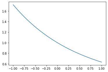
The plot suggests that:
This is possible because whilst both the numerator and denominator tend to zero they do so at exactly the same rate (like \(x/x\)). In the next section we will learn how to find limits of this type.
6.2.1. Limit definition of \(e^x\)#
Recall from our earlier work on exponentials that the natural exponent \(e\) satisfies
From this expression we can obtain
This is one of many ways that can be used to define and calculate the exponential function (though it converges quite slowly). Taking \(n=10^7\) gives the value of \(e\) correct to 5 decimal places:
n=10**7
print((1+1/n)**n)
2.7182816941320818
6.3. Asymptotic equivalence#
Whereas the limit of a function refers to tendency towards a single value, asymptotic equivalence refers to tendency towards a relationship.
In the last chapter we learned how to construct asymptotes for rational fractions as \(x\to \pm\infty\). For example, returning to (6.1), for large positive \(x\) the function has
a limit of negative infinity
an asymptote \(y=-\frac{3x}{2}-\frac{7}{4}\).
We can develop deeper theory that allows us to construct asymptotically equivalent polynomials for almost any sort of continuous function and in almost any limit. This is one of the most important ideas in mathematics, because it allows us to find approximate analytic solutions to problems that may otherwise be too challenging to solve. Most commonly we are interested in results that are valid in the limit as \(x\) tends to zero.
We haven’t yet studied the required mathematical theory to construct asymptotic expansions from scratch, but we will return to this later in the module. For now, we merely state results for some common functions or obtain them using Python, without justification.
Useful polynomial approximations (power series)
For “very small” \(x\), the following expressions are asymptotically equivalent. In most practical applications we only need the first two or three terms.
Exercise 6.4
Using the result given above, write down the first three terms in the power series expression for \((1+x)^{1/2}\). Estimate the maximum relative error in this expansion over the range \([-0.2,0.2]\).
Using the given expansion formula,
We can calculate the relative error for a list of values in the given range:
import numpy as np

x = np.linspace(-0.2,0.2,100)
y_asy = 1 + x/2 - x**2/8
y_act= (1+x)**(1/2)
err = (y_asy - y_act)/y_act
It is a good idea to plot the relative error, to check for any odd behaviour, such as discontinuities. Here we plot the absolute value as we are interested in the relative size of the error and not the direction:
import matplotlib.pyplot as plt
plt.plot(x,np.abs(err))
plt.show()
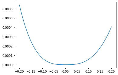
There is no odd behaviour here. We can see that the largest relative error on the range occurs when \(x=-0.2\), and is about 0.064%.
100*max(np.abs(err))
0.0640419931155935
Exercise 6.5
The sinc function appears often in engineering applications. It is defined for \(x\neq 0\) by
What do you think is the value of this function in the limit \(x\rightarrow 0\) ?
It is useful to plot the function:
import numpy as np
import matplotlib.pyplot as plt

x = np.linspace(-4*np.pi,4*np.pi,100)
y= np.sin(x)/x

plt.plot(x,y)
plt.show()
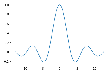
By inspecting the graph we are led to conclude that in the limit \(x\rightarrow 0\) the function approaches a finite value (one?) from both sides. Let’s see if we can verify this algebraically.
We can make use of the power series expression for \(\sin(x)\) given above:
Therefore we have formally shown that
The sinc function is undefined as \(x=0\), but we can adjust the definition to take care of the hole discontinuity as follows:
6.4. A little help from Python#
We can use the sympy library to find limits or asymptotically equivalent power series. The two expressions you can use to explore a function \(y(x)\) as \(x\rightarrow x_0\) are:
limit(y,x,x0)series(y,x,x0,n)
The second expression gives the \(n\) term power series. For example,
from sympy import *
x = symbols('x')
series((1-exp(x))/(2*x),x,0,3)
\(\displaystyle -\frac{1}{2}-\frac{x}{4}-\frac{x^2}{12}+\mathcal{O}(x^3)\)
series((1-exp(-2*x))/x,x,0,3)
\(\displaystyle 2-2x+\frac{4x^2}{3}+\mathcal{O}(x^3)\)
We can verify these results using the given power series for \(e^x\). For instance:
We can also infer the following limits using the series expansions:
\(\begin{alignat}{5} &\lim_{x \to 0}\frac{1-e^x}{2x} &&=\lim_{x\to 0}\left(-\frac{1}{2}+\mathcal{O}(x)\right)=-\frac{1}{2}\\ &\lim_{x\to 0}\frac{1-e^{-2x}}{x} &&=\lim_{x\to 0}\left(2+\mathcal{O}(x)\right)=2 \end{alignat}\)
Exercise 6.6
Find an \(\mathcal{O}(x)\) power series expansion for the following function, and deduce the limit as \(x\) tends to zero:
\(\qquad \displaystyle y=\frac{\sqrt{1-x^2}-\sqrt{1+x}}{x}\).
For small \(x\)
Therefore,
In the limit:
You can verify this using the following code:
from sympy import *
x = symbols('x')
series((sqrt(1-x**2)-sqrt(1+x))/x,x,0,2)
Exercise 6.7
Find an \(\mathcal{O}(1/x)\) power series expansion for the following function, and deduce the limit as \(x\) tends to infinity:
\(\qquad \displaystyle\lim_{x \to \infty} \big( \sqrt{x^2-2} - \sqrt{x^2+x} \big)\).
Where we require an asymptotic result for \(f(x)\) as \(x\to \infty\), this is equivalent to \(f(\frac{1}{y})\) as \(y\to 0^+\).
Introducing \(y=1/x\) gives
This is identical to the problem we solved in [2]. Therefore the series expansion is given by
and the limit is \(-1/2\). You can verify the result again using Python:
from sympy import *
x = symbols('x')
series(sqrt(x**2-1)-sqrt(x**2+x), x, oo, 2)
6.5. Do limits always exist?#
Not all functions have a limit at all points. For example, consider the square root function \(\sqrt{x}\), which is not real-valued for \(x<0\). This function only has a limit from the right at \(x=0\) and does not have a limit for negative values of \(x\).
A more exotic example is given by the function shown in Fig. 6.1. The function oscillates faster approaching zero and does not approach a particular value, so it does not have a limit as \(x\to 0\).
import numpy as np
import matplotlib.pyplot as plt

x = np.linspace(-1,1,10000)
y = np.sin(1/x)
plt.plot(x,y)
plt.show()
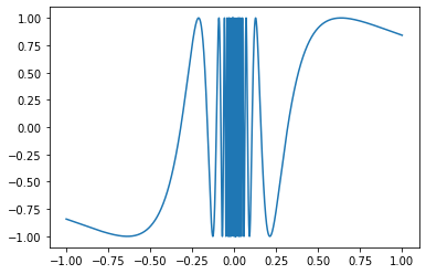
Fig. 6.1 A plot of the function \(\sin(1/x)\).#
Exercise 6.8
Do either of the following limits exist?
The first limit exists and is equal to 0.
The second limit does not exist.
6.6. Limiting sums#
The power series expansions that we saw above are examples of infinite sums. Although we usually keep only the first few terms in these sums, we can in principle keep going in the expansion up to arbitrarily high powers of \(x\). It may be difficult to believe that when we add an infinite number of terms we can obtain a finite result. However, a relatively simple example may convince you of this fact.
Consider the sum below, containing \(n\) terms:
In mathematical notation this would usually be written as follows, representing the sum from \(k=1\) to \(n\) of the given expression :
A curious person could investigate this sum by calculating a result for the first few values of \(n\). We could even plot the results to see if there is a visible pattern:
r=1/4
t=[r**k for k in range(1,20)] #terms in series

import numpy as np
s=np.cumsum(t)                #running total

import matplotlib.pyplot as plt
plt.plot(s,'o')
plt.show()
print(s)
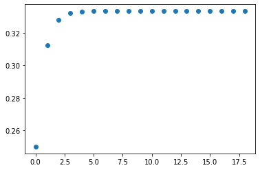
The plot gives the impression that the sum is approaching a constant value. If you try increasing the value of \(n\) you will find that the result numerically settles down (converges) to 0.33333333.
Warning
This result is not a proof. Sometimes a sum that that appears to be numerically converging to a finite limit may in fact be growing to infinity at an extremely slow rate, as demonstrated in the following example. Conversely, a sum that appears to be growing extremely large may be converging towards an extremely large (but finite) limit.
Sometimes the sympy library in Python may be able to give us the limit of a sum \(S_n\) as the number of terms \(n\) tends to infinity. We can do it here for the sum given in (6.6). The result agrees with our numerical estimate:
from sympy import *
k = Symbol('n', integer=True)
r=1/4
Sum(r**k,(k,1,oo)).doit()
0.333333333333333
For this example we can understand the result graphically. We consider a unit square partitioned as shown below. The total shaded area represents the sum, and we can see from the picture that the result is finite. We can also note that for every shaded square there are two unshaded squares of the same size, so the shaded region represents 1/3 of the total area of the square.
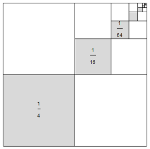
Fig. 6.2 A graphical representation of \(\displaystyle\sum_{k=1}^{\infty}\left(\frac{1}{4}\right)^k\)#
The sum we just considered is an example of a geometric sum, which means that it has the form
We can find a general result for sums of this type using algebra. We do this by cross-elimination of terms:
\(\begin{alignat}{5} S_n &= a + && ar+ar^2+\dots +ar^{n-1}\\ r S_n &= && ar+ar^2+\dots +ar^{n-1}+ar^n\\ \implies (1-r)S_n &= a- && ar^n\\ &&&\implies S_n = \frac{a(1-r^n)}{1-r} \end{alignat}\)
If \(r<1\) then as \(n\to \infty\), \(r^n\to 0\) and so we obtain the famous geometric series formula:
For example, when \(r=1/4\), the result is \(S_\infty=1/3\).
Warning
It is important to give here a word of warning about infinite sums. If the terms in the sum shrink to zero in the limit, this is not sufficient to guarantee convergence. A counter-example is provided below.
Consider now the famous “harmonic series”, which is given by:
Notice that the terms in this sum converge to zero:
Therefore you might expect that the sum would converge to a finite limit. Indeed, after a million terms the sum has still not exceeded a value of 15:
t=[1/k for k in range(1,1000000)]
import numpy as np
s=np.cumsum(t)

import matplotlib.pyplot as plt
plt.plot(s)
plt.show()
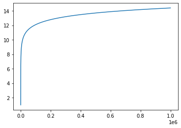
After 100 million terms the sum still has not exceeded 20. However, we can prove that this sum does not converge to a finite limit by grouping together the terms as shown:
This latter sum grows without bound.