Accumulating change
Contents
10. Accumulating change#
pp67 Modeling Life
Even in the late 1940s and 1950s numerical integration was still frequently done by hand. Hodgkin and Huxley used it to do their simulation of the firing of a neuron, for which they received the Nobel Prize. In the early years of the US space program, human computers - many of whom were African-American women with math degrees but limited employment options - worked in aeronautical engineering at [NASA]. The book Hidden Figures [tells] their story (Shetterly 2016).
10.1. Numeric solution#
Consider a general equation of the following form, where \(f(x,t)\) is a known function:
To obtain a numeric estimate of the solution we can use the discrete derivative formula
where \(h\) is the step size of \(t\). By using this formula to estimate the continuous derivative in (10.1) we the may obtain the rearrangement
This allows us to start from a given initial value \(x_0\) and “step forward” successively to obtain \(x_1\), \(x_2\), etc.
10.1.1. Example#
Consider the equation governing exponential growth/decay:
The discrete formula for this problem is given by
Notice that the solution grows if \(\alpha>0\), which matches what we expect to see for exponential growth.
The code below can be used to carry out the forward stepping and plot the solution. By comparing to the known solution we can find the size of the error on a given interval. Here, using a step size \(h=0.02\), the maximum error is also around 0.02%.
import numpy as np
import matplotlib.pyplot as plt

a=0.1 #alpha

#range of values to plot for
t=np.linspace(0,20,10000)

#initialise solution array
x=np.ones(len(t))

# forward stepping
h=t[1]-t[0] #step size

for i in range(len(t)-1):
  x[i+1] = (1+a*h)*x[i]

plt.plot(t,x)
plt.show()

# Calculate the error using the known solution
x_sol=np.exp(a*t)
err=(x-x_sol)/x_sol

# Maximum error (as %)
print(100*max(abs(err)))
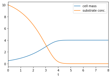
Exercise 10.1
Numerically solve Monod’s model (9.5) for the following parameters to plot the substrate concentration and cell mass:
\(\mu_{max}=0.75\text{l/h}\), \(K_s=2\text{mg/l}\), \(Y=0.35\), \(S_0=10\text{mg/l}\), \(X_0=0.5\text{mg/l}\).
import matplotlib.pyplot as plt
import numpy as np

mu=0.75; K=2;  Y=0.35; S0=10; X0=0.5

def model(X):
  S=S0-(X-X0)/Y
  return mu*S*X/(K+S)

tmax=8;
t=np.linspace(0,tmax,1000)

X = np.ones(len(t)); X[0]=X0; #pre-allocate
h = t[1]-t[0]

for i in range(len(t)-1):
  X[i+1]=X[i]+h*model(X[i])

plt.plot(t,X,label='cell mass')
plt.plot(t,S0-(X-X0)/Y,label='substrate conc.')
plt.legend()
plt.xlim([0,tmax])
plt.xlabel('t')
plt.show()
10.2. Integration#
Brief