16. Climate tipping points

Getting tipsy

Climate tipping points are conditions beyond which changes in a part of the climate system become self-perpetuating. These changes may lead to abrupt, irreversible, and dangerous impacts with serious implications for humanity.

This case study is provided for you to understand how mathematical models can give insight about system behaviour. You will be introduced to a dynamic model of Earth’s energy balance, which you will use to identify tipping point phenomena.

To accompany this case study you are recommended to watch the Mathematical Association of America lecture by Mary Lou Zeeman, co-director of the Mathematics and Climate Research Network.

16.1. Naked planet model

The naked planet model is a model of Earth’s energy balance that ignores the effect of the atmosphere. It is a simple one-stock model in which the Earth is warmed by the suns rays and radiates the additional heat back to space.

16.1.1. Energy inflow

The Earth is warmed by energy radiated from the sun onto the facing surface area. The rate of incoming energy from the sun is known as the solar constant. It can be measured by satellites above the Earth’s atmosphere and is found to be roughly \(1361\text{W/m}^2\). Although for historic reasons it is known as a constant, the incoming energy does vary over the solar cycle, and over the long-term life of the sun.

Note

One watt is equal to one joule of energy per second.

Not all of the energy received by the Earth is absorbed. Some of the incoming solar radiation is reflected back to space, for example due to cloud cover or due to the reflectivity of Earth’s surfaces. More energy is absorbed by the oceans than by land, and areas that are covered by snow and ice have higher reflectivity than green forest.

The fraction of energy that is reflected is known as albedo. It can be estimated by satellite imaging, as shown in the figure below. From such observations the Earth’s average albedo is estimated to be around 29.5%.

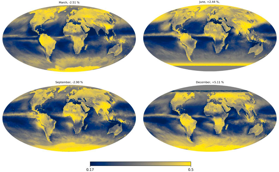
Fig. 16.1 The spherical albedo of the Earth. Darker and bluer values indicate lower albedo, brighter and more yellow values higher albedo. [paper]

The inflow of energy at Earth’s surface is therefore estimated by

(16.1)\[Q_{in} = \pi R^2 L(1-\alpha),\]

where \(R\) is the radius of Earth, \(L\) is the solar constant, \(\alpha\) is the albedo (fraction reflected). In this formula, \(\pi R^2\) is the area of Earth perpendicular to the sun’s rays. Multiplying this area by \(L\) gives the solar energy, and multiplying by \((1-\alpha)\) gives the amount absorbed.

16.1.2. Energy outflow

The rate of energy radiated from the Earth’s surface to space is estimated from the blackbody radiation law:

\[\begin{equation*} Q_{out} = 4\pi R^2\sigma T^4, \end{equation*}\]

where \(\sigma\) is the Stefan-Boltzmann constant. In this formula, \(4\pi R^2\) is the surface area of the Earth and \(\sigma T^4\) is thermal radiation per square metre at a temperature of \(T\) Kelvin.

16.1.3. Rate of change

The rate of energy absorption per unit area is given by

\[\begin{equation*} \frac{\mathrm{d}Q}{\mathrm{d}t}=\frac{Q_{in}-Q_{out}}{4\pi R^2}=\frac{L(1-\alpha)}{4}-\sigma T^4. \end{equation*}\]

The rate of change of temperature is related to the rate of energy absorption by the effective heat capacity of Earth, \(C\simeq 0.53\text{GJm}^{-2}\text{K}^{-1}\), which gives

(16.2)\[C\frac{\mathrm{d}T}{\mathrm{d}t}=\frac{L(1-\alpha)}{4}-\sigma T^4\]

A summary of the parameter values is given in the table below, for convenience. To be consistent with these units, time is measured in seconds. If we want to measure time in years, we multiply the right hand side of (16.2) by the number of seconds in one year.

Table 16.1 Summary of parameters in the naked planet model. Values shown in green are for Earth.

Symbol	Represents	Value	Units
\(\sigma\)	Stefan-Boltzmann constant	\(5.67\times 10^{-8}\)	\(\text{W/m}^2\text{K}^4\)
\(\alpha\)	Albedo	\(0.295\)	—
\(C\)	Effective heat capacity	\(5.3\times 10^8\)	\(\text{Jm}^{-2}\text{K}\)
\(L\)	Solar constant	\(1361\)	\(\text{W/m}^2\)
\(T\)	Temperature of the planet	?	\(K\)

Exercise 16.1

Solve the climate model (16.2) for \(T(0)=250\) and for \(T(0)=260\), and plot the solutions on the same figure. Ensure that the axes are correctly labelled, with the units included.

You should find that the solution approaches an equilibrium value, which is the same in both cases.

16.1.4. Equilibrium

When the inflow and outflow are balanced, the model is in equilibrium and the temperature remains constant. The equilibrium value is at the intersection of the inflow and outflow curves plotted below.

import numpy as np
import matplotlib.pyplot as plt

a = 0.295   #Albedo
s = 5.67e-8 #Stefan-Boltzmann constant
L = 1361    #Solar constant

Tmax=300 #set plot range

T = np.linspace(0,Tmax,1000)

inflow  = L*(1-a)/4  #constant
outflow = s*T**4

plt.plot(T,outflow,'r',label='inflow')
plt.plot([0,Tmax],2*[inflow],'b',label='outflow')
plt.xlim([0,Tmax])
plt.ylim([0,max(outflow)])
plt.xlabel('Temp /K')
plt.legend()
plt.show()

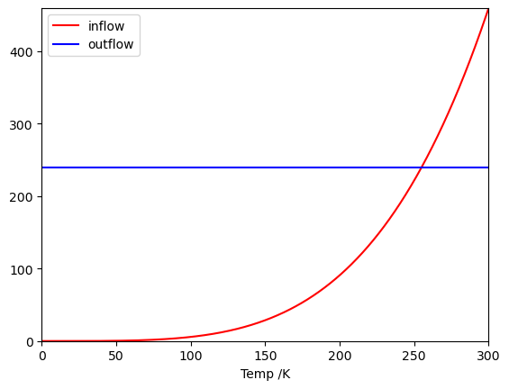
Fig. 16.2 The equilibrium temperature is at the intersection between the inflow and outflow energy curves. Here, the energy is measured in \(\text{W/m}^2.\)

Exercise 16.2

Find the equilibrium temperature in Celsius, based on (16.2). Comment on your answer.

16.2. Greenhouse effect

The interior of a greenhouse (glass house) warms up more than its surroundings because it traps heat. Glass is fairly transparent to incoming short-wave solar radiation, but is much less transparent to the long-wave radiation that is re-emitted from surfaces in the greenhouse such as soil and plants.

The atmosphere of Earth behaves in similar manner to the glass of a greenhouse, which results in less heat emitted to space than what the naked earth model predicts. Today it is possible to directly observe the greenhouse effect by comparing the amount of Earth’s heat radiated from the upper atmosphere to the amount leaving the surface, but the idea that CO2 in the Earth’s upper atmosphere could result in atmospheric warming appears to have been first suggested in 1856 by Eunice Newton Foote.

We can amend the naked earth model to account for the greenhouse effect by multiplying the long wave radiation term by a fraction \(1/(1+g)\) that reduces the amount of short wave radiation outflow:

(16.3)\[C\frac{\mathrm{d}T}{\mathrm{d}t}=\frac{L(1-\alpha)}{4} -\frac{\sigma T^4}{1+g}\]

When \(g=0\) we have the naked Earth model. It can be shown that when \(g=1\) the equilibrium state of the model is equivalent to a hypothetical model of the Earth contained within a glass ball. Values of \(g>1\) can be used to model a “super greenhouse effect”.

Exercise 16.3

The 20th century average temperature of Earth was about 13.9°C. By taking this to be the equilibrium state of model (16.3), estimate the value of the greenhouse parameter \(g\).

16.3. Ice albedo feedback

At colder temperatures the earth would be covered in snow and ice, resulting in a higher albedo. An example model of how the albedo changes with temperature is shown below.

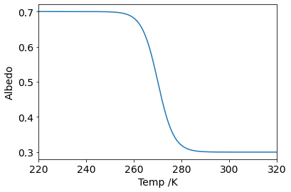
Fig. 16.3 At frozen temperatures the albedo (reflectivity) of Earth is high. In the model, the snowball Earth thaws between 263K and 283K.

Exercise 16.4

Write a function albedo that resembles the above figure by using a scaled and shifted sigmoid

\[\begin{equation*} \alpha(T) = A+\frac{(B-A)e^{k(T-T_m)}}{1+e^{k(T-T_m)}} \end{equation*}\]

for appropriate choices of \(A,B,k,T_m\).

16.4. Investigation

By including both the effects of ice-albedo feedback and the greenhouse effect in model (16.3), investigate the equilibrium state of the planet at follows:

Exercise 16.5

Suppose the earth starts in “Goldilocks” equilibrium state described in Exercise 16.3. Describe what happens to the equilibrium state of the system as \(g\) decreases, with reference to the tipping point. What are the approximate values of \(g,T\) at the tipping point?

Exercise 16.6

Suppose that the Earth is in a snowball state with \(g\sim 0.5\) and \(T\sim 227\text{K}\). Explain what is required to happen in this model for Earth to return to the Goldilocks state.