Fitting curves
Contents
4. Fitting curves#
“with four parameters I can fit an elephant, and with five I can make him wiggle his trunk”.
This chapter illustrates how curves can be fitted to data to estimate the values of theoretical parameters. After completing this chapter you should be able to fit a specified function to a numerical dataset and use the obtained coefficients in further calculations.
The curve fitting in this chapter is done by the method of least squares, which aims to minimise the sum of the squared residual errors between the fitted function and the data.
4.1. Global temperature anomaly#
Loosely speaking, radiative forcing refers to the amount of additional solar energy (Watts per square metre, Wm-2) absorbed by the Earth due to climate factors.
An estimate of radiative forcing due to atmospheric \(\ce{CO2}\) concentrations was given by the Swedish scientist Svante Arrhenius, who received the Nobel prize for Chemistry in 1903. The relationship can be written in the following form
where \(\alpha\) is a constant,
\(C\) is the atmospheric concentration of \(\ce{CO2}\) at time \(t\)
\(C_0\) is the atmospheric concentration of \(\ce{CO2}\) at reference time
\(\Delta F\) is the amount of additional solar energy due to radiative forcing
Exercise 4.1
Estimates have placed the value of \(\alpha\) in (4.1) at around 5.35Wm-2 for Earth’s atmosphere. Calculate the amount of additional solar energy due to radiative forcing between pre-industrial levels (CO2 approx 275ppm) to present day (CO2 approx 410ppm).
Multiplying \(\Delta F\) by the Earth’s total area gets the total warming energy in Watts. This results in a figure that is approximately 60 times larger than the global annual energy consumption (~18TW). But what impact does it have on temperature?
We will assume that the change in temperature \(\Delta T\) is linearly proportional to the increase in energy, which we may write as:
The value of the constant \(\hat{\alpha}\) may be estimated from data.
Exercise 4.2
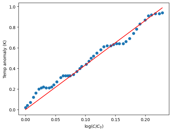
The dataset climate-change-2.csv shows \(\ce{CO2}\) levels (\(C\)) alongside the global temperature anomaly \(\Delta T\). Produce a plot of \(\Delta T\) against \(\ln(C/C_0)\), taking \(C_0\) to be the first value in the dataset.
Data for this question were obtained from ourworldindata.org.
Code to import and plot the datapoints is given below
import matplotlib.pyplot as plt
import pandas as pd
import numpy as np

#import the data
df = pd.read_csv('climate-change-2.csv')
C=df['CO2 (ppm)']
y=df['Temp anom (K)']

x=np.log(C/C[0])     #x=log(C/C0)
plt.plot(x,y,'o')    #plot

#prettify
plt.xlabel("log($C/C_0$)")
plt.ylabel("Temp anomaly (K)")
plt.show()
We can fit the function \(y=\hat{\alpha} x\) to the data to estimate the value of \(\hat{\alpha}\) in (4.2). This is done below using the scipy.optimize library:
# function to fit, with unknown parameters
def func(x,a):
  return a*x

from scipy import optimize
coeffs=optimize.curve_fit(func,x,y)[0]
alpha_hat = coeffs[0]
print("alpha_hat = " , alpha_hat)
alpha_hat = 4.3208138030469385
A plot of the fitted line together with the curve is shown below:
plt.plot(x,y,'o')
xx=np.array([0,max(x)])
plt.plot(xx,alpha_hat*xx,'r')

#prettify
plt.xlabel("log($C/C_0$)")
plt.ylabel("Temp anomaly (K)")
plt.show()
Exercise 4.3
Use the calculated value of \(\hat{\alpha}\) to produce a crude estimate of how much higher global average surface temperatures will be compared to pre-industrial levels if \(\ce{CO2}\) levels rise to twice pre-industrial levels.
Taking \(C/C_0=2\) and \(\hat{\alpha}=4.321\) in (4.2) gives \(\Delta T=2.99^{\circ}C\).
This result is within the range of estimates produced by the Intergovernmental Panel on Climate Change [IPCC].
4.2. Radiation therapy#
Radiation therapy aims to treat cancers by exposure to radiation. The SI unit for a dose of absorbed radiation is the “Gray” (Gy), corresponding to the absorption of 1joule of radiation per kg of matter. Higher levels of radiation exposure result in greater clinical effect, but also increased damage to surrounding tissues.
In a research paper on Mathematical Modelling of Radiotherapy Strategies for Early Breast Cancer, an electron-beam driven x-ray source was used to deliver radiation to a taget site. The following experimental values were quoted in the research paper, illustrating how the amount of radiation at the site depends on the distance between the x-ray source and the target:
distance (cm) |
dose (Gy) |
|---|---|
0.1 |
15.00 |
0.2 |
12.50 |
0.5 |
8.75 |
1.0 |
5.00 |
2.7 |
1.00 |
Exercise 4.4
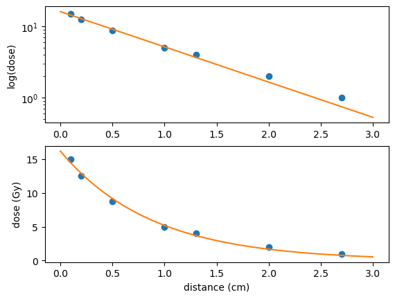
Demonstrate graphically that the (distance,dose) data approximately fits the function \(y=A e^{k x}\), and find values of the constants \(A,k\) that give a good fit.
To demonstrate that \((x,y)\) data approximately fit an exponential relationship we can show that a plot of \(\log(y)\) against \(x\) follow a linear trend. This can be understood by taking the log of both sides of the exponential relationship:
The relationship is of the form \((Y=kx+c)\), where \(Y=\log(y)\) and \(c=\log(A)\).
To find the constants we could either :
fit a straight line to the \(\log(y)\) data
fit the exponential function to the \(y\) data
The two approaches are not equivalent due to the statistical way that curve fitting is done. However, they will give similar results.
Here, the exponential fit has been carried out using the scipy.optimize library:
import matplotlib.pyplot as plt
import numpy as np

x = np.array([0.1,0.2,0.5,1.0,1.3,2.0,2.7])
y = np.array([15.00,12.50,8.75,5.00,4.00,2.00,1.00])

from scipy import optimize

def func(x,A,k):                          #exponential function to fit
  return A*np.exp(k*x)

coeffs=optimize.curve_fit(func,x,y)[0]    #best fit for y

xx=np.linspace(0,3,100)                   #values for plot
yy=func(xx,*coeffs)                       #apply fit to xx values

fig, axs = plt.subplots(2,1)
axs[0].semilogy(x,y,'o',xx,yy)
axs[1].plot(x,y,'o',xx,yy)
axs[1].set_xlabel('distance (cm)')
axs[0].set_ylabel('log(dose)')
axs[1].set_ylabel('dose (Gy)')
plt.show()
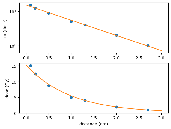
For comparison the results of the linear fit approach are shown below. Only the curve fitting part of the code needs to be replaced with
def func(x,k,c):                               #linear function to fit
  return k*x+c

coeffs=optimize.curve_fit(func,x,np.log(y))[0] #best fit for log(y)

xx=np.linspace(0,3,100)                        #values for plot
yy=np.exp(func(xx,*coeffs))                    #apply fit to xx values
The polyfit function from the numpy library can also be used to fit a straight line. However, this function can only be used to fit polynomials and is therefore less powerful than scipy.optimize. Its use is exemplified below:
c = np.polyfit(x,np.log(y),1) #fit a degree 1 polynomial
yy=np.exp(c[1]+c[0]*xx)       #convert log(y) --> y
A dose of radiation is often delivered in smaller amounts called fractions. This can allow healthy cells to repair sub-lethal damage to their DNA between fractions. A treatment plan may be developed that depends on the type of cancer and proximity to organs.
The clinical effect of treatment can be modelled by the following “Linear-Quadratic” (LQ) relationship
where \(D\) is the total dose, \(d\) is the dose per fraction, \(n\) is the number of fractions. The first term represents lethal damage due to single-hit double strand chromsome breaks, and the second term represents lethal damage due to a combination of two sub-lethal single strand chromasome breaks. The coeffcicients \(\alpha\), \(\beta\) depend on the tumour site and histology. Notice that if the same dose \(D\) is delivered in a larger number of fractions (thereby reducing \(d\)) the clinical effect \(E\) is reduced, with the amount of sparing depending on the \(\alpha/\beta\) ratio.
By assuming that lethal damage is Poisson distributed with rate constant \(E\), we obtain that the probability of cell survival is given by
Clinical data on radiotherapy often refers to one of two quantities related to the clinical effect, which are EQD2 and BED. These quantifications are used to compare a given treatment plan to either the equivalent dose required in 2Gy fractions (EQD2) or the effective hypothetical dose if the treatment was delivered over an infinite number of “zero fractions” (BED).
For EQD2 we may write
For BED we may write
These two quantities have sometimes been confused in published research papers, which could have serious prescription consequences.
Read more
If you want to read more about this model, see (for example)
Exercise 4.5
The following experimental parameter values were quoted in the research paper on Mathematical Modelling of Radiotherapy Strategies for Early Breast Cancer:
\(\begin{alignat*}{5} &\bullet\ \text{Tumour: }\quad &&\alpha=0.30,\quad &&\alpha/\beta=10\\ &\bullet\ \text{Tissue: } &&\alpha=0.15, &&\alpha/\beta=3 &\end{alignat*}\)
Use these values to estimate the BED (4.6) and survival probabilities (4.4) for a single dose of radiation at each of the following doses (Gray):
Your calculated values should approximately match those given in Table 1 of the research paper.
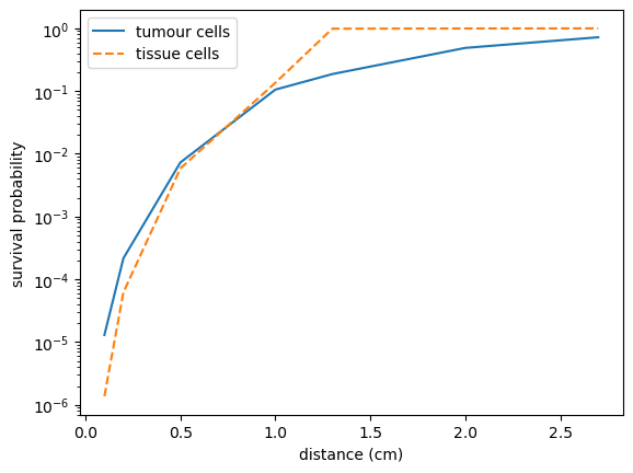
If you wish, you can also calculate \(S^*_{tissue}\) according to equation (2b) in the paper, and therefore reproduce Figure 4 from the paper.
We can apply the given formulae as follows:
import numpy as np

dvals = np.array([15.00,12.50,8.75,5.00,4.00,2.00,1.00])

# definitions
def radioth(d,a,b):
  BED=d*(1+d/(a/b)); S=np.exp(-a*BED);
  return [BED,S]

a1=0.30; b1=a1/10;              #tumour
[BEDtum,Stum]=radioth(dvals,a1,b1)

a2=0.15; b2=a2/3;               #tissue
[BEDtis,Stis]=radioth(dvals,a2,b2)
You can then use print to display the results.
The following code can be used to calculate the adjusted probabilities. The zip function is used here to apply the adjst function to the pairs of values defined by the arrays dvals and Stis
# adjust S for tissue repair
def adjst(d,S):
  if d<5:
    S=S+0.98*(d<5)*(1-S)
  return S

Ssta=[adjst(d,S) for (d,S) in zip(dvals,Stis)]

import matplotlib.pyplot as plt
x = np.array([0.1,0.2,0.5,1.0,1.3,2.0,2.7])

plt.semilogy(x,Stum,label='tumour cells')
plt.semilogy(x,Ssta,'--',label='tissue cells')
plt.xlabel('distance (cm)')
plt.ylabel('survival probability')
plt.legend()
plt.show()
Here are the results:
Dose_ |
BED_a |
S_tumour |
BED_b |
S_tissue |
S*tissue |
|---|---|---|---|---|---|
15.00 |
37.50 |
1.30e-05 |
90.00 |
1.37e-06 |
1.37e-06 |
12.50 |
28.12 |
2.17e-04 |
64.58 |
6.21e-05 |
6.21e-05 |
8.75 |
16.41 |
7.29e-03 |
34.27 |
5.85e-03 |
5.85e-03 |
5.00 |
7.50 |
1.05e-01 |
13.33 |
1.35e-01 |
1.35e-01 |
4.00 |
5.60 |
1.86e-01 |
9.33 |
2.47e-01 |
9.85e-01 |
2.00 |
2.40 |
4.87e-01 |
3.33 |
6.07e-01 |
9.92e-01 |
1.00 |
1.10 |
7.19e-01 |
1.33 |
8.19e-01 |
9.96e-01 |
4.3. Earthquakes#
The calmag.txt dataset contains 18,402 Richter scale measurements for magnitude 3+ earthquakes that were recorded in California from 1960 to 2014. The smallest and largest recorded values were 3.0 and 7.3 respectively. These data were downloaded from the U.S Geological Survey www.usgs.gov.
We can produce a histogram of this data as shown below. The hist function produces a histogram, and also outputs the frequencies n and edge values bin.
import numpy as np
import matplotlib.pyplot as plt

calmag = np.loadtxt("data/calmag.txt")
n, bin, _ = plt.hist(calmag, bins=40)

plt.xlabel('Magnitude M / Richter')
plt.ylabel('Frequency')
plt.show()
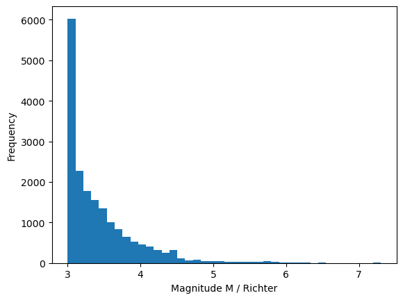
Fig. 4.2 Frequency of Richter magnitude earthquakes in California, 1960-2014#
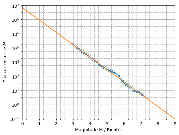
The Gutenberg-Richter (GR) law predicts that in any given region and time period, the number of earthquakes that are at least Richter magnitude \(x\) is given by the following relationship, where \(\alpha,\beta\) are constants:
Therefore a plot of \(\ln(N_x)\) against \(x\) is expected to follow a decreasing linear trend.
Exercise 4.6
Use the n, bin values calculated above to produce a plot of \(\ln(N_x)\) against \(x\) and fit a trendline to the data. Do the data support the GR law?
Hint: what result is given by np.cumsum(n[::-1])[::-1] ?
Taking the natural logarithm of the proposed relationship gives
In the below code I used polyfit to obtain the trendline, but you could also use scipy.optimize. The data appear to fit the GR law very well!
x=bin[0:-1]                        #ignore rightmost edge
Nx = np.cumsum(n[::-1])[::-1]      #reverse cumsum
plt.semilogy(x,Nx,'x')             #plot the data

#fit and plot the trendline
coeffs=np.polyfit(x,np.log(Nx),1)
xx=np.array([0,9])
yy=np.exp(coeffs[0]*xx+coeffs[1])
plt.semilogy(xx,yy)

plt.xlim([0,9])
plt.xlabel('Magnitude M / Richter')
plt.ylabel('# occurrences $\geq M$')
plt.show()
Exercise 4.7
According to the GR law with the parameters we calculated, how many magnitude 8+ earthquakes can be expected in a 30 year period?
Hint: The expected number of earthquakes is a value less than one.
By assuming that magnitude 8+ earthquakes are Poisson-distributed, estimate the probability of a magnitude 8+ earthquake occurring in the next 30 years in California.
Hint: Taking \(X\sim\text{Po}(\lambda)\) where the expected number of events is \(\lambda\), the probability of no events is given by
beta = -coeffs[0]
alpha = np.exp(coeffs[1])

# Expected number of earthquakes in data time period
N8=alpha*np.exp(-beta*8)

# The dataset covers a 54 year period, so in 30 years:
L=N8*30/54
print("Expectation of 8+ earthquakes in 30 years",L)

# Pr(x>0) = 1-Pr(x=0)
p=1-np.exp(-L)
print("Estimated probabilty : {0:.1%}".format(p))
Expectation of 8+ earthquakes in 30 years 0.39837
Estimated probabilty : 32.9%
Warning
We should be extremely careful when making estimates based on extrapolation beyond the domain of the available data. A comic illustration of this warning can be found at https://xkcd.com/1007/
4.4. Heart rate monitoring#
Many wearable devices allow heart rate and activity data to be tracked and downloaded as txt or csv files. It may be possible to estimate circadian rhythms from this data.
The hrdata2.csv dataset contains “fitbit” measurements of activity and heart rate (HR) for a single individual, obtained from a recent research paper. The data are for a period of 96 hours, averaged every five minutes. The HR is measured in beats per minute (bpm), and the activity level is measured in steps per minute.
The heart rate can be modelled by the equation
where \(\mu\) is the average background HR, \(A\) is the amplitude of the 24hr circadian cycle, and \(\epsilon\) is statistical error (e.g. due to measurement inaccuracies).
The activity effect \(E(a)\) is the increase in HR due to activity \(a\). To estimate the background circadian rhythm, we will attempt to remove the activity effect from the data.
We begin by selecting the data for waking periods only. Plotting the activity \(a\) against \((\text{HR}-\mu)\) shows the effect of the activity.
Due to background noise and circadian variation there is a wide band of HR measurements, which need to be statistically averaged. Doing this calculation is beyond the scope of the course, so the activity effect has been estimated for you. The Activity_effect column in the dataset gives the estimated effect size \(E(a)\). The predicted relationship is plotted below in red, with the measured data shown in blue.
import matplotlib.pyplot as plt
import pandas as pd
import numpy as np

#import the data
df = pd.read_csv('hrdata2.csv')

# get waking data
df=df.loc[df['Sleep'] == False]
df=df.sort_values(by='Activity')

#average resting waking heart rate
mu=np.mean(df.loc[df['Activity']==0,'HR'])
print("Resting HR (awake) : ",mu)

x=df['Activity']           #activity
y=df['HR']-mu              #adjusted HR
z=df['Activity_effect']    #activity effect

plt.plot(x,y,'o')          #(activity,HR data)
plt.plot(x,z,'r')          #(activity,effect) estimates

#prettify
plt.xlabel('Activity, a')
plt.ylabel('HR effect, E(a)')
plt.show()
Resting HR (awake) : 62.71232876712329
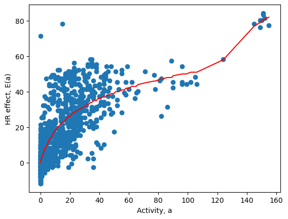
Fig. 4.3 Heart rate increase due to activity (bpm)#
The plot suggests that the effect of additional activity on HR is not linear. The good news is that light activity such as a gentle walk results in an appreciable heart rate effect. At a level of just 20 steps per minute this person’s HR increased by around 20bpm. However, further increases in activity level resulted in a smaller HR effect until around 100 steps per minute (a moderate walk). At more vigorous levels of activity corresponding to a vigorous walk or light jog we again start to see greater effect of additional activity. Can you use your knowledge of the cardiovascular system to suggest why this might be?
Exercise 4.8
Using the given dataset, plot the adjusted HR against time.
On the same axes, plot the curve
where \(A,\mu\) are “best fit” estimates for the data.
import matplotlib.pyplot as plt
import pandas as pd
import numpy as np

#import the data
df = pd.read_csv('hrdata2.csv')
t=df['Sec']/60          #time
y=df['HR_adjusted']     #adjusted heart rate


#plot the data
plt.plot(t,y,'k',label='data')

# Fitted curve
from scipy.optimize import curve_fit

def func(t, mu, A):
    return mu + A*np.sin(np.pi*t/12.0)

coeffs = curve_fit(func, t, y)[0]
print(coeffs)

tfit = np.linspace(0,96,100)
yfit = func(tfit,*coeffs)
plt.plot(tfit,yfit,'r',label='fit')

#prettify
plt.xlabel('time (hrs)')
plt.ylabel('Heart rate (bpm)')
plt.xlim([0,96])
plt.legend()
plt.show()
[61.56597222, 4.04033287]
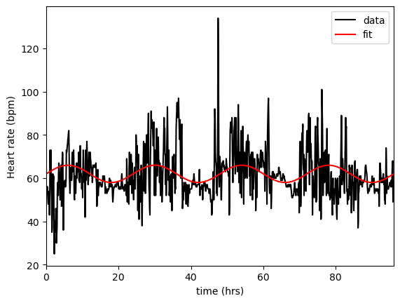
Although the plotted data still contains a large amount of variation/noise, we appear to have done a reasonable job of identifying a circadian rhythm, with the basal heart rate for this person being around 61-62bpm with a daily (resting) variation of \(\pm\)4bpm.
In their research paper, the authors found that the circadian rhythms for some of their volunteers did not align with the sleep-wake cycle. For instance, one of their participants was undertaking shift work, but their daily heart-rate cycle remained aligned to a standard day/night pattern.