Viral trends solutions

Exercise 13.1

Use the code given in the homework sheet to import the data :

import pandas as pd
import numpy as np

df = pd.read_csv('data_2022-Aug-17.csv')
df=df.iloc[::-1] #data in reverse order

x=np.array(df['date'])
y=np.array(df['newCasesBySpecimenDate'])

from datetime import date as dt
date=dt.fromisoformat
dt0 = date(x[0])
x=[abs(date(x[i])-dt0).days for i in range(len(x))]

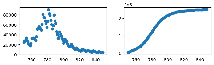
Isolate a wave “by eye” and find the running total number of cases

import matplotlib.pyplot as plt

x=np.array(x[750:850])
y=np.array(y[750:850])

fig, ax = plt.subplots(1, 2,figsize=(8,2))
ax[0].plot(x,y,'o')

#subtracting baseline number of cases
Y = np.cumsum(y-min(y))
ax[1].plot(x,Y,'o')
plt.show()

Define the logistic function

def logistic_fun(x,K,x0,s):
  return K/(1+np.exp(-(x-x0)/s))

Note

It is possible to fit the function without normalising, but to do this we have to help the optimizer locate the parameter values by providing bounds.

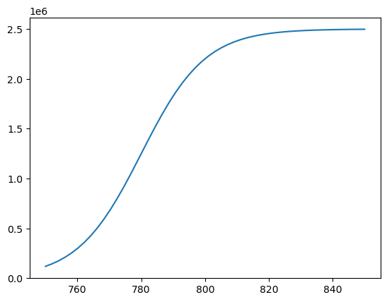
We can identify suitable parameter bounds by trying out some coefficient values in the logistic function until we get some that look roughly correct:

xtest = np.linspace(750,850)
ytest = logistic_fun(xtest,2.5e6,780,10)
plt.plot(xtest,ytest)
plt.show()

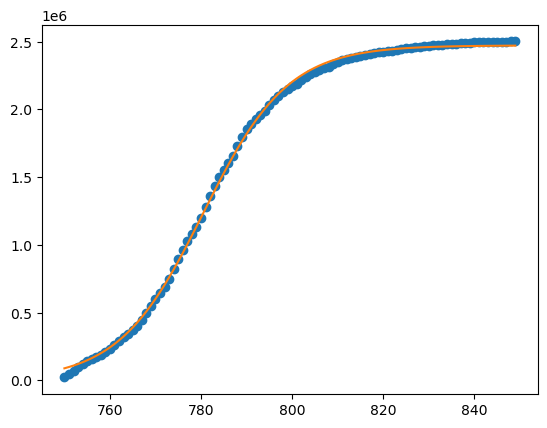
Provide coefficient bounds that span the indicated values:

from scipy.optimize import curve_fit
bds=((1e6,760,1),(5e6,840,100))
params=curve_fit(logistic_fun,x,Y,bounds=bds)[0]
print(params) # these are the values we found

# plot the result :
plt.plot(x,Y,'o')
Y_fit=logistic_fun(x,*params)
plt.plot(x,Y_fit)
plt.show()

The homework suggested to normalize the data. You could plot the result after the following step, to check correctness:

def my_normalize(v):
  a=min(v); b=max(v)
  vhat=(v-a)/(b-a)
  return vhat,a,b

xhat,L,R = my_normalize(x)
Yhat,D,U = my_normalize(Y)

Now fit the logistic function. You could plot the result after the following step, to check correctness:

from scipy.optimize import curve_fit

params=curve_fit(logistic_fun,xhat,Yhat)[0]
Yhat_fit=logistic_fun(xhat,*params)

To “un-normalise” we perform the reverse of the normalization steps:

def un_normalize(vhat,a,b):
  return vhat*(b-a)+a

Yfit = un_normalize(Yhat_fit,D,U)
plt.plot(x,Y,'o')
plt.plot(x,Yfit)
plt.show()

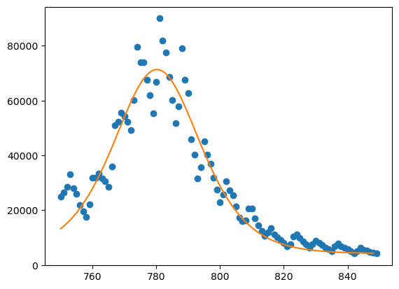
Finally, to plot the daily cases we reverse the accumulation step

yfit = np.diff(Yfit)+min(y)
plt.plot(x,y,'o')
plt.plot(x[0:-1],yfit)
plt.show()

Exercise 13.2

Import the call me maybe data

import pandas as pd
import numpy as np
df = pd.read_csv('call-me-maybe.csv')
x=np.array(df['week'])
h=np.array(df['hits'])
y=np.cumsum(h)           #accumulate  

Note

Again, we can do the fit without normalising if we tinker with the parameters to establish suitable bounds:

def frechet(x,A,k,s):
  y=A*np.exp(-(x/k)**(-s))
  return y

from scipy.optimize import curve_fit
bds=((1e3,50,2),(1e4,500,10))
params=curve_fit(frechet,x,y,bounds=bds)[0]
print(params)

Yfit = frechet(x,*params)

import matplotlib.pyplot as plt
plt.plot(x,y,'b.')
plt.plot(x,Yfit)
plt.show()

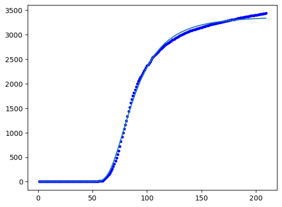
With normalisation:

# normalise
xhat=x/len(x)
yhat=y/max(y)

# curve fit
from scipy.optimize import curve_fit
import matplotlib.pyplot as plt

def frechet(x,k,s):
  return np.exp(-(x/k)**(-s))

bds=((0.01,0.01),(1,100))
params=curve_fit(frechet,xhat,yhat,bounds=bds)[0]
print(params)

Yfit = frechet(xhat,*params)

plt.plot(xhat,yhat,'b.')
plt.plot(xhat,Yfit)
plt.show()

Showing the weekly hits :

yfit = np.diff(max(y)*Yfit)
plt.plot(x,h,'b.')
plt.plot(x[0:-1],yfit)
plt.show()

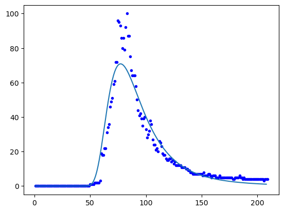
The distribution pdf has a similar shape to the data (variance, skeweness) but a lower peak (kurtosis).