Linear systems
Contents
23. Linear systems
Now, we will start to build up some theory. To do this, we will revert to the simplest general class of 2D problem, which consists of a pair of coupled, linear differential equations. We will consider a system of the form
The equation can be written in matrix form as follows:
Recalling the ansatz for systems of this type, we may take \((x,y)=(x_0 e^{\lambda t},y_0 e^{\lambda t})\), and by substituting into the ODE we obtain
This is an eigenvalue problem \(A\underline{x}=\lambda \underline{x}\), where \(A\) is the coefficient matrix. We may distinguish the character of the phase portrait according to the nature of the eigenvalues.
We will consider some examples below. In each example, the phase portrait will be plotted on the range \(x,y\in[-2,2]\). We start by making the a meshgrid for this domain.
import numpy as np
import matplotlib.pyplot as plt

x=np.linspace(-2, 2, 10)
y=np.linspace(-2, 2, 10)
X,Y = np.meshgrid(x, y)
23.1. Real, distinct eigenvalues \(\lambda_1 \neq \lambda_2\)
First we will consider some examples where the eigenvalues are real and distinct. In that case, the general form of the solution can be written as
in which \(\underline{v}_1,\underline{v}_2\) are eigenvectors corresponding to the eigenvalues \(\lambda_1,\lambda_2\), and \(c_0,c_1\) are arbitrary constants, which may be chosen to satisfy any given initial conditions.
Notice that as \(t\rightarrow\infty\) one of the eigensolutions will dominate and so solution trajectories will end up parallel to the eigenvector corresponding to the largest eigenvalue.
Eigenvector directions
According to the relationship \(A\underline{x}=\lambda\underline{x}\), the vector field at points lying along the eigenvector directions points directly away/towards the equilibrium point at the origin, depending on the sign of the eigenvalue.
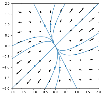
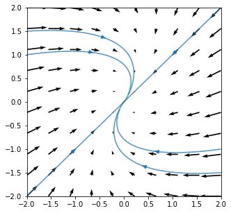
23.1.1. Unstable node: \(\lambda_1, \lambda_2 >0\)
Consider the following example system :
The eigenvalues and corresponding eigenvectors of the coefficient matrix are given below. The direction \(y=x\) has the largest eigenvalue and solution trajectories will end up parallel to this direction.
All solution trajectories point away from the equilibrium point, which is unstable.
#define the vector field values at each point
(U,V)=(4*X+Y,2*X+3*Y)

fig,ax=plt.subplots(figsize=(5,5))
ax.axis([-2,2,-2,2])
ax.quiver(X,Y,U,V)

#----------------------------------
start=[ #start points of selected field lines
    [-0.1,-0.1],[0.1,0.1],[-0.1,0.2],[0.1,-0.2],
    [0,1],[1,0],[0,-1],[-1,0],
    [0,2],[2,0],[0,-2],[-2,0]
    ]
#----------------------------------
ax.streamplot(X,Y,U,V,start_points=start,density=20)
plt.show()
Exercise 23.1
Write down the general solution of the given ODE
The general form of the solution is
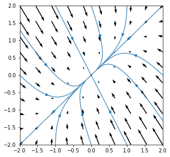
23.1.2. Stable node: \(\lambda_1, \lambda_2<0\)
Consider the following example system :
The eigenvalues and corresponding eigenvectors of the coefficient matrix are given below. The direction \(y=-2x\) has the largest (magnitude) eigenvalue and solution trajectories will be parallel to this direction for large negative \(t\)
All solution trajectories point towards the equilibrium point, which is stable.
#define the vector field values at each point
(U,V)=(-2*X+Y,2*X-3*Y)

fig,ax=plt.subplots(figsize=(5,5))
ax.axis([-2,2,-2,2])
ax.quiver(X,Y,U,V)

#----------------------------------
start=[ #start points of selected field lines
    [-0.1,0.2],[0.1,-0.2],[-0.1,-0.1],[0.1,0.1],
    [1,0],[-1,0],[-1,-2],[1,2],
    [0,2],[2,0],[0,-2],[-2,0]
    ]
#----------------------------------
ax.streamplot(X,Y,U,V,start_points=start,density=20)
plt.show()
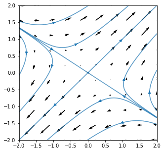
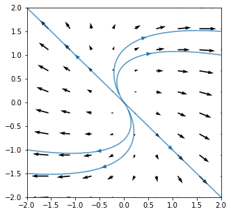
23.1.3. Saddle: \(\lambda_1<0\), \(\lambda_2>0\)
In the example below there is one positive eigenvalue and one negative. The solution trajectory approaches one of the trajectories as \(t\rightarrow-\infty\) and the other as \(t\rightarrow +\infty\).
#define the vector field values at each point
(U,V)=(X+3*Y,2*X+2*Y)

fig,ax=plt.subplots(figsize=(5,5))
ax.axis([-2,2,-2,2])
ax.quiver(X,Y,U,V)

#----------------------------------
start=[ #start points of selected field lines
    [-0.1,-0.1],[0.1,0.1],[-2,+4/3],[+2,-4/3],
    [-2,4/3-0.01],[-2,4/3-0.2],[-2,4/3+0.01],[-2,4/3+0.2],
    [2,-4/3+0.01],[2,-4/3+0.2],[2,-4/3-0.01],[2,-4/3-0.2]
    ]
#----------------------------------
ax.streamplot(X,Y,U,V,start_points=start,density=20)
plt.show()
Exercise 23.2
Calculate the eigenvalues and corresponding eigenvectors for this problem.
Eigenvalues and corresponding eigenvectors:
23.2. Real repeated eigenvalues \(\lambda\)
If the eigenvalue problem has repeated roots \(\lambda\) corresponding to eigenvector \(\underline{v}_1\) then we need to find a second linearly independent solution. We may try the following ansatz
Substituting into the problem \(\underline{x}^{\prime}=A\underline{x}\) we find this is a solution if
Thus, the general solution is of the form
For large \(t\) the term \(t\underline{v}_1e^{\lambda t}\) dominates and the solution ends up parallel to the eigenvector \(\underline{v}_1\)
23.2.1. Unstable inflected node: \(\lambda>0\)
Eigenvalues and corresponding eigenvectors:
#define the vector field values at each point
(U,V)=(3*X+Y,-X+Y)

fig,ax=plt.subplots(figsize=(5,5))
ax.axis([-2,2,-2,2])
ax.quiver(X,Y,U,V)

#----------------------------------
start=[ #start points of selected field lines
    [-0.1,0.1],[0.1,-0.1],[2,1],[-2,-1],[2,1.5],[-2,-1.5]]
#----------------------------------
ax.streamplot(X,Y,U,V,start_points=start,density=20)
plt.show()
Exercise 23.3
Find the general solution of the given ODE
Solve \((A-\lambda I)\underline{v}_2=\underline{v}_1\), where \(\underline{v}_1=\begin{bmatrix}1\\-1\end{bmatrix}\)
A suitable choice is \(\underline{v}_2=\begin{bmatrix}0\\1\end{bmatrix}\)
The general form of the solution is
23.2.2. Stable inflected node: \(\lambda<0\)
The following problem is an example of a stable inflected node. See if you can sketch it.
Solution
Eigenvalues and corresponding eigenvectors:
23.3. Complex conjugate eigenvalues \(\lambda=\mu\pm i\omega\)
In the case of complex conjugate eigenvalues the eigenvectors will also be complex, of the form \(\underline{v}=\underline{v}_r\pm i\underline{v}_i\). Expanding out the complex terms in the general solution (23.3) using Euler’s identity gives a solution of the form
where
It can be seen that the solutions for \((x,y)\) demonstrate oscillating behaviour with growing or decay amplitude.
You may also recall earlier from earlier work on eigenvalues and eigenvectors that real eigenvectors correspond to a stretch transform and that complex eigenvalues correspond to a rotation transform. In the phase plane, the change vectors \(A\underline{x}\) are rotational.
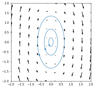
23.3.1. Centre: \(\mu=0\)
In the case where the eigenvalues are purely imaginary, the solution oscillates without change of amplitude. The equilibrium point is neutrally stable. If we perturb the system away from its equilibrium point it will not return to equilibrium, but neither will it move away from it. The solution will remain on a trajectory encircling the equilibrium point.
Eigenvalues : \(=\pm 2i\)
#define the vector field values at each point
(U,V)=(Y,-4*X)

fig,ax=plt.subplots(figsize=(5,5))
ax.axis([-2,2,-2,2])
ax.quiver(X,Y,U,V)

#----------------------------------
start=[ #start points of selected field lines
    [0.1,0.1],[0.3,0.3],[0.6,0.6]]
#----------------------------------
ax.streamplot(X,Y,U,V,start_points=start,density=20)
plt.show()
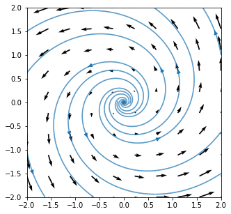
23.3.2. Unstable spiral: \(\mu>0\)
The following system is an example case where the equilibrium point is an unstable spiral. The eigenvalues are complex conjugate, so the solutions oscillate. Since the real part of the eigenvalue is positive, the amplitude of the oscillations grows ever-larger. An example of a system demonstrating this type of behaviour would be a pendulum with “negative friction”.
Eigenvalues : \(\lambda=1\pm 3i\)
#define the vector field values at each point
(U,V)=(X-3*Y,3*X+Y)

fig,ax=plt.subplots(figsize=(5,5))
ax.axis([-2,2,-2,2])
ax.quiver(X,Y,U,V)

#----------------------------------
start=[ #start points of selected field lines
    [0.1,0.0],[0,0.1],[-0.1,0],[0,-0.1],[2,1],[-2,-1],[2,-1.5],[-2,1.5]]
#----------------------------------
ax.streamplot(X,Y,U,V,start_points=start,density=20)
plt.show()
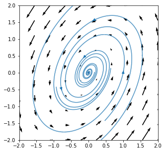
23.3.3. Stable spiral \(\mu<0\)
Exercise 23.4
Find the eigenvalues of this system and have a go at plotting the phase portrait by hand. Verify your answer by producing a computer plot of the phase portrait. You could do this either by showing the vector field with a few streamlines, or by plotting the solution trajectory for suitable initial conditions
You could also have a try at finding the general form of the solution, although we do not need it to construct the phase portrait.
Solution:
Eigenvalues : \(\lambda=-\frac{1}{2}(1\pm \sqrt{51}i)\)
In the code below the solution phase portrait is constructed from the vector field. Have a try at plotting solution trajectories using odesolve.
23.4. Summary
In two dimensions we can encounter a range of equilibrium types:
Nodes and saddle points (stable or unstable) are a superposition of 1d equilibrium types
Spirals and centres are an irreducibly 2d type of equilibrium, because they involve rotation
The derivations here were done for linear systems, but in the next chapter we will see that these types of equilibrium point can also be encountered in nonlinear systems.
Exercise 23.5
The Rayleigh model is given by
Produce a phase portrait for this system for some different values of the constant \(c\). Try values that are negative, positive and zero. How does the character of the equilibrium point change?
Solution:
There is an equilibrium point at \((0,0)\). Some illustrative phase portraits are shown below.
For \(c<-2\) it is a stable node
For \(-2<c<0\) it is a stable spiral
For \(0<c<2\) it is an unstable spiral
For \(c>2\) it is an unstable node
The critical values where the equilibrium point changes type are:
When \(c=-2\) it is a stable inflected node
When \(c=0\) it is a centre
When \(c=2\) it is an unstable inflected node
fig,ax=plt.subplots(2,2,figsize=(10,10),)

x = np.linspace(-2,2,1000)
y = np.linspace(-2,2,1000)
[X,Y] = np.meshgrid(x,y)

c=-1
(U,V)=(Y,-X-c*(Y**3-Y))
start=[[0.5,0.5],[1,1]]
ax[0,0].streamplot(X,Y,U,V,start_points=start,density=20,arrowsize=2)
ax[0,0].set_title('c=-1')

c=0
(U,V)=(Y,-X-c*(Y**3-Y))
start=[[0.5,0.5],[1,1]]
ax[0,1].streamplot(X,Y,U,V,start_points=start,density=20,arrowsize=2)
ax[0,1].set_title('c=0')

c=1
(U,V)=(Y,-X-c*(Y**3-Y))
start=[[0.5,0.5],[1,1]]
ax[1,0].streamplot(X,Y,U,V,start_points=start,density=20,arrowsize=2,maxlength=10.0)
ax[1,0].set_title('c=1')


c=2.1
(U,V)=(Y,-X-c*(Y**3-Y))
start=[[0.5,0.5],[-0.5,-0.5],[0.5,-0.5],[-0.5,0.5],[1,1]]
ax[1,1].streamplot(X,Y,U,V,start_points=start,density=20,arrowsize=2,maxlength=10.0)
ax[1,1].set_title('c=3')
plt.show()
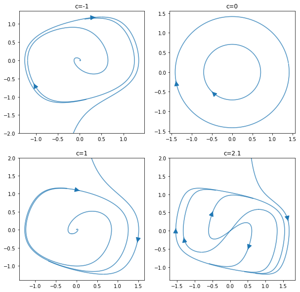
Notice also that there is a limit cycle, which is unstable for \(c<0\) and stable for \(c>0\).
23.5. Equilibrium points in \(n\) dimensions
Equilibrium points in \(n\) dimensions are composed of the 1d and 2d types that we have considered - i.e. nodes,spirals and centres. For example, consider the following system, which has an equilibrium point at the origin
The system has one real eigenvalue, which is negative and two that are positive
from numpy import linalg as la

M=np.array([[3,-9,8],[7,-4,-4],[-5,4,1]])
k, v = la.eig(M)

for i in k:
  print(i)
(0.08016923561500475+10.296566482037464j)
(0.08016923561500475-10.296566482037464j)
(-0.16033847123000597+0j)
Hence, the equilibrium point combines the 2d behaviour of a stable centre with the 1d behaviour of a stable node.
Here, plotting the 2d phase portrait at a constant value of \(z\) shows the stable spiral
x=np.linspace(-10, 10, 10)
y=np.linspace(-5, 5, 10)
z=np.linspace(-5, 5, 10)
X,Y,Z = np.meshgrid(x, y, z)

#define the vector field values at each point
(U,V,W)=(3*X-9*Y+8*Z,7*X-4*Y-4*Z,-5*X+4*Y+Z)

start=[[0.1,0.1]]

plt.streamplot(X[:,:,5],Y[:,:,5],U[:,:,5],V[:,:,5],start_points=start,density=20)
plt.show()
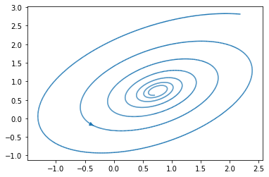
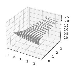
Plotting one of the solution trajectories can illustrate the nature of the equilibrium point in three dimensions:
init=np.real(4*v[:,2]+[1,1,0])

def mysys(X,t):
  dXdt=np.matmul(M,X)
  return dXdt

t = np.linspace(0, 10, 101)

from scipy.integrate import odeint
sol = odeint(mysys,init, t)

fig = plt.figure()
ax = plt.axes(projection='3d')
ax.plot3D(sol[:,0], sol[:,1], sol[:,2], 'gray')
plt.show()