.md .pdf

Contents

5. Variations of Fields

5.1. Divergence

If we start with a vector field \({\bf A(r)} = A_x({\bf r})\,\hat{\bf x} + A_y({\bf r})\,\hat{\bf y} + A_z({\bf r})\,\hat{\bf z} \), then we can define the quantity \(\nabla\cdot {\bf A(r)}\), i.e. taking the scalar product of the gradient operator with vector field \({\bf A(r)} \) which since the gradient vector is a differential operator, means the expression has the form:

\[\nabla\cdot {\bf A(r)} = \partial_x\, A_x + \partial_y\, A_y + \partial_z\, A_z\]

This is often known as the Divergence of \({\bf A(r)}\) or \(\text{div}\,{\bf A(r)}\). Note that in the case of operators we need to be a little careful of the ordering of the terms, since \({\bf A(r)}\cdot \nabla\) would give:

\[{\bf A(r)} \cdot \nabla= A_x\,\partial_x + A_y\,\partial_y + A_z\,\partial_z \]

which is also a differential operator, waiting to act on another term, which we apply on the right.

Lets see the effect of this on two vector fields \({\bf A_1(r)} = \begin{pmatrix} x \\ y \\ 0\end{pmatrix}, \,{\bf A_2(r)} = \begin{pmatrix} y \\ -x \\ 0\end{pmatrix}\):

\[\begin{split}\nabla \cdot {\bf A_1} &= \partial_x\, x + \partial_y\, y + \partial_z\, 0 = 2 \\ \nabla \cdot {\bf A_2} &= \partial_x\, y - \partial_y\, x + \partial_z\, 0 = 0 \end{split}\]

which we can visualise in Fig. 5.1.

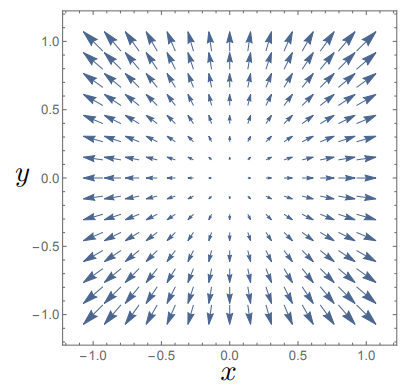
Fig. 5.1 Plotting the vector field \({\bf A_1}\) which has non-zero divergence.

We can see that the origin here really plays the role of a centre of the divergence, the field lines all appear to flow outwards, becuase here \(\nabla \cdot {\bf A} > 0\). In the case of \(\nabla \cdot {\bf A} < 0\), field lines would flow into a point and there would be a convergnece of the field.

5.2. Curl

We can likewise take a vector field $\({\bf A(r)} \) and here take the vector product with the gradient operator \(\nabla\times {\bf A(r)}\), which has components:

\[\begin{split}\nabla\times {\bf A(r)} = \begin{pmatrix} \partial_y\, A_z - \partial_z\, A_y \\ \partial_z\, A_x - \partial_x\, A_z \\ \partial_x\, A_y - \partial_y\, A_x \end{pmatrix}\end{split}\]

which is know as the Curl or Rotation of the vector field \(\bf A(r)\) or \(\text{curl}\,{\bf A(r)}\).

To see the effects of these, lets consider again \({\bf A_1(r)} = \begin{pmatrix} x \\ y \\ 0\end{pmatrix}, \,{\bf A_2(r)} = \begin{pmatrix} y \\ -x \\ 0\end{pmatrix}\):

\[\begin{split}\nabla \times {\bf A_1} &= \begin{pmatrix} \partial_y\, 0 + \partial_z\, x \\ \partial_z\, y - \partial_x\, 0 \\ \partial_x\, y - \partial_y\, x \end{pmatrix} = \begin{pmatrix} 0 \\ 0 \\ 0 \end{pmatrix} \\ \nabla \times {\bf A_2} &= \begin{pmatrix} \partial_y\, 0 + \partial_z\, x \\ \partial_z\, y - \partial_x\, 0 \\ \partial_x\, x + \partial_y\, y \end{pmatrix} = \begin{pmatrix} 0 \\ 0 \\ 2 \end{pmatrix}\end{split}\]

which we can visualise in Fig. 5.2.

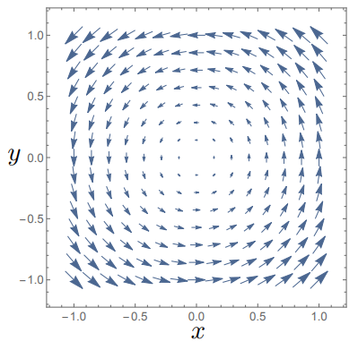
Fig. 5.2 Plotting the vector field \({\bf A_2}\) which has non-zero curl.

We note that “centre” of this rotation is at the origin and that \(\nabla \times {\bf A_2}\) points in the \(z\) direction. We define this rotation as following the right hand rule, depicted in Fig. 5.3, curling the fingers on our right hand around and the thumb pointing in the direction of the vector.

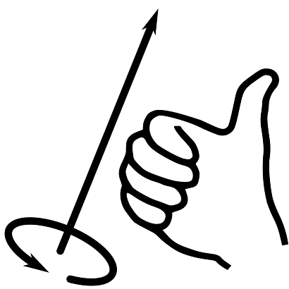
Fig. 5.3 The right hand rule for a curl field

We can see that a linear combination of vector fields \(\bf A_1 + A_2\) would produce a vector field with both divergence and curl, which is shown in Fig. 5.4.

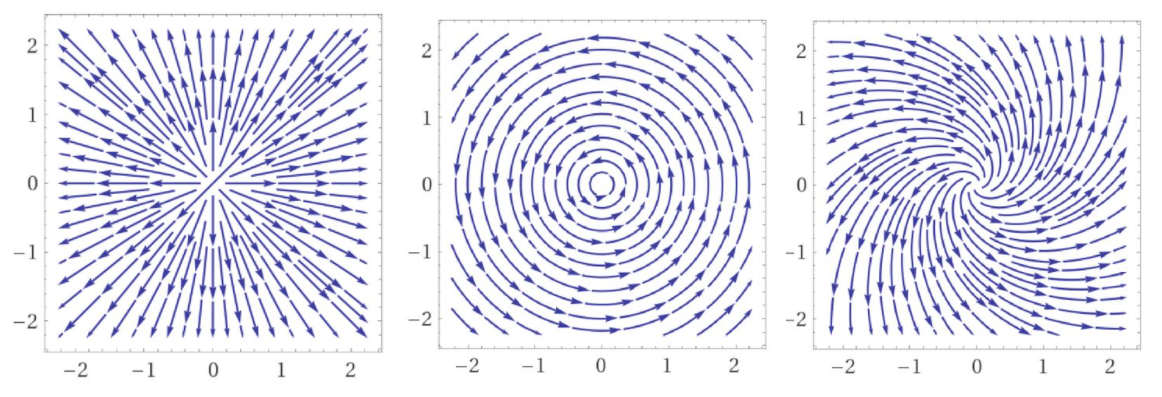
Fig. 5.4 The effect of adding a divergence (curl free) field to a curl (divergence free) field.

We can use the product rule as well as the rules following scalar and vector products to find a vareity of vector calculus relations:

\[\begin{split}\nabla(\phi\,\psi) &= \psi(\nabla \phi) + \phi(\nabla \psi)\\ \nabla \cdot(\phi {\bf A}) &= (\nabla \phi)\cdot {\bf A} + \phi(\nabla \cdot {\bf A})\\ \nabla \times(\phi {\bf A}) &= (\nabla \phi)\times {\bf A} + \phi(\nabla \times {\bf A})\\ \nabla \cdot ({\bf A \times B}) &= (\nabla \times {\bf A})\cdot {\bf B} - {\bf A}(\nabla \times\cdot {\bf B})\\ \nabla \times ({\bf A \times B}) &= (\nabla \cdot {\bf B} + {\bf B}\cdot \nabla)\,{\bf A} - (\nabla \cdot {\bf A}+ {\bf A}\cdot \nabla)\,{\bf B}\end{split}\]

5.3. 2nd Order Variations of Fields

We can combine two or more gradients in a vector expression, one of the most useful is to find the divergence of the gradient of a scalar field \(\phi\),

\[\textrm{div grad} \,\phi = \nabla \cdot (\nabla \phi) = \nabla^2 \phi = (\partial_x^2 + \partial_y^2 + \partial_z^2)\phi\]

This is sometimes also written as \(\Delta\phi = \nabla^2 \phi \) and is known as the Laplacian of \(\phi\).

We can also find the divergence of the curl of a vector field:

\[\text{div}\,\,\text{curl}\,{\bf A} = \nabla \cdot (\nabla \times {\bf A}) = 0\]

which holds for all vector fields. Thinking again about the fields shown in Fig. 5.4,w e can think of these two processes as complementary, rotation around a point compared with emergence from / convergence to a point.

Likewise if we look at the curl of a gradient field:

\[\text{curl}\,\,\text{grad}\,\phi = \nabla \times \nabla \phi = 0\]

which is true for all scalar fields.

In general we can write a vector field as having two sets of components, one curl free and one divergence free, this is known as the Helmholtz Decomposition of a vector field:

\[{\bf B} = -\nabla \phi + \nabla \times {\bf A}\]

previous

4. Vector Fields

next

6. Coordinate Systems