24. Bifurcation analysis¶

In this section we will start to examine systems with more than one equilibrium point. We will also allow that the systems may contain parameters and we will consider how the number of equilibrium points and their stability changes as parameter values are varied.

To assist our analysis we will introduce an analytic method for classifying equilibrium points of nonlinear systems (linearisation). We will also introduce the idea of a bifurcation diagram as a way of representing our findings.

24.1. Linearisation¶

We now consider a general first order coupled autonomous system involving two dependent variables. The problem may be written in the following form, in which the arbitrary functions \(f\) and \(g\) may be nonlinear:

(24.1)¶\[\begin{align} \dot{x} & = f(x,y)\\ \dot{y} & = g(x,y) \end{align}\]

We will assume that the system has an equilibrium point \((x_0,y_0)\) satisfying

(24.2)¶\[\begin{equation} f(x_0,y_0)=g(x_0,y_0)=0. \end{equation}\]

Finding equilibria

It is not always possible to find all equilibrium points by hand if \(f,g\) are not both simple algebraic functions. In such cases a numerical root-finding algorithm such as Newton-Raphson or bisection algorithm could be employed.

To examine the nature of the equilibrium point, we will expand the functions \(f\) and \(g\) using Taylor series centred at \((x_0,y_0)\). Since we are interested in the behaviour of solution trajectories in the neighbourhood of the point, we can linearise the expansion:

(24.3)¶\[\begin{align} f(x,y) & = f(x_0,y_0) +(x-x_0)\frac{\partial f}{\partial x}\biggr|_{(x_0,y_0)}+(y-y_0)\frac{\partial f}{\partial y}\biggr|_{(x_0,y_0)}+\dots\\ g(x,y) & = g(x_0,y_0) +(x-x_0)\frac{\partial g}{\partial x}\biggr|_{(x_0,y_0)}+(y-y_0)\frac{\partial g}{\partial y}\biggr|_{(x_0,y_0)}+\dots\\ \end{align}\]

We can further simplify by making the variable substitution \(X=(x-x_0)\), \(Y=(y-y_0)\) to obtain

(24.4)¶\[\begin{align} \dot{X} &= X\frac{\partial f}{\partial x}\biggr|_{(x_0,y_0)}+Y\frac{\partial f}{\partial y}\biggr|_{(x_0,y_0)}\\ \dot{Y} &= X\frac{\partial g}{\partial x}\biggr|_{(x_0,y_0)}+Y\frac{\partial g}{\partial y}\biggr|_{(x_0,y_0)} \end{align}\]

This is a first order linear system in two unknowns, with equilibrium point at \((X,Y)=(0,0)\). We can write it in matrix form, just as we did in the previous chapters:

(24.5)¶\[\begin{equation} \frac{\mathrm{d}}{\mathrm{d}t}\begin{bmatrix}X\\Y\end{bmatrix} = J(x_0,y_0)\begin{bmatrix}X\\Y\end{bmatrix}, \qquad J(x_0,y_0)= \begin{bmatrix}\frac{\partial f}{\partial x} & \frac{\partial f}{\partial y}\\ \frac{\partial g}{\partial x} & \frac{\partial g}{\partial y}\end{bmatrix}_{(x_0,y_0)} \end{equation}\]

The coefficient matrix \(J(x,y)\) is called the Jacobian. Finding the eigenvalues and eigenvectors of the Jacobian at the stationary point tells us its stability and allows us to plot the shape of the solution trajectories.

24.1.1. Example: Nonlinear pendulum¶

Recall the equation for the undamped pendulum that was given in the Section 22.2 :

(24.6)¶\[\begin{align} \dot{x} & = y && =f(x,y)\\ \dot{y} & = -\omega^2 \sin(x) && =g(x,y) \end{align}\]

Equilibrium points:

(24.7)¶\[\begin{equation} f=g=0 \qquad \Rightarrow \quad x=n\pi, \ n\in\mathbb{Z} \end{equation}\]

Evaluate the Jacobian:

(24.8)¶\[\begin{equation} J(x,y) = \begin{bmatrix}\frac{\partial f}{\partial x} & \frac{\partial f}{\partial y}\\ \frac{\partial g}{\partial x} & \frac{\partial g}{\partial y}\end{bmatrix} = \begin{bmatrix}0 & 1\\ -\omega^2\cos(x) & 0\end{bmatrix} \end{equation}\]

We can separate treatment of the equilibrium points according to even and odd \(n\).

At \(x=n\pi\) (\(n\) even)

\(J(2m\pi,0) = \begin{bmatrix}0 & 1\\-\omega^2 & 0 \end{bmatrix}\)

Eigenvalues: \(\lambda=\pm i\omega\) (centres)

At \(x=n\pi\) (\(n\) odd)

\(J((2m+1)\pi,0) = \begin{bmatrix}0 & 1\\\omega^2 & 0 \end{bmatrix}\)

Eigenvalues: \(\lambda=\pm \omega\) (saddles)

This agrees with the results we found earlier by plotting the vector field and solution trajectories.

Exercise 24.1

The equation of motion for the damped pendulum is given by

\[\begin{align*} \dot{x}& = y\\ \dot{y} & = -\omega^2 \sin(x)-ky \\ \end{align*}\]

Find and classify the equilibrium points, using the linearisation technique. You may assume that \(k,\omega\) are both positive.

Solution

The equilibrium points are at \(x=n\pi\), as for the stable case.

For \(n\) even the eigenvalues are \(\lambda=\frac{1}{2}\left(-k\pm \sqrt{k^2-4\omega^2}\right)\)

For \(n\) odd the eigenvalues are \(\lambda=\frac{1}{2}\left(-k\pm \sqrt{k^2+4\omega^2}\right)\)

Since \(\sqrt{k^2+4\omega^2}>k\) \(\forall\omega\neq 0\), the odd nodes are always saddles. The classification of the even nodes depends on the value of \(k\), with \(k=2\omega\) being a critical value.

For \(k<2\omega\) (underdamped), the points are stable spirals
For \(k>2\omega\) (overdamped), the points are stable nodes

24.2. Differential equations with a parameter¶

The exercise above involved a parameter \(k\). Other sections of the notes have also featured examples that involved parameters. For example,

Exercise 22.2 featured parameters \(c,k\)
Exercise 23.5 featured parameter \(c\)

We have seen that it is possible for the behaviour of the system change as the parameter is varied. In some cases changing one parameter can result in a transition from having a stable equilibrium to an unstable one, or vice-versa. We saw this in the glycolysis example. In other cases there may also be equilibrium states that exist only within certain parameter regimes.

We will now attempt to systematically study how the location and stability of any equilibria vary for different parameter values.

24.2.1. Example: A pitchfork bifurcation¶

To illustrate the approach, let us consider the following system that features parameter \(\mu\) :

(24.9)¶\[\begin{align} \dot{x} &=y &&=f(x,y)\\ \dot{y}&=\mu x - y - x^3-x^2 y &&=g(x,y) \end{align}\]

Equilibrium points are found at \((0,0)\), \((\pm\sqrt{\mu},0)\), with the latter points existing only for \(\mu\geq 0\). To classify the equilibrium points we use the Jacobian, which is given by

(24.10)¶\[\begin{equation} J(x,y)=\begin{bmatrix}0 & 1\\ \mu-3x^2-2xy & -1-x^2\end{bmatrix} \end{equation}\]

At \((0,0)\) the eigenvalues are

\[\begin{equation*} \lambda = \frac{1\pm \sqrt{1+4\mu}}{2} \end{equation*}\]

This equilibrium point is:

stable spiral for \(\mu<-1/4\)
stable inflected node at \(\mu=-1/4\)
stable node for \(-1/4<\mu<0\)

At \((\pm\sqrt{\mu},0)\) the eigenvalues are

\[\begin{equation*} \lambda =\frac{-(1+\mu)\pm \sqrt{\mu^2-6\mu+1}}{2} \end{equation*}\]

This equilibrium point is:

stable node for \(0<\mu<3-2\sqrt{2}\)
stable inflected node for \(\mu=3\pm2\sqrt{2}\)
stable spiral for \(3-2\sqrt{2}<\mu<3+2\sqrt{2}\)
stable node for \(\mu>2+2\sqrt{2}\)

This information can be represented on a bifurcation diagram, in which we represent the parameter \(\mu\) on the horizontal axis and the \(x\)-location of the equilibrium point(s) on the vertical axis. A solid line is used to represent a stable equilibrium and a dashed line is used to represent an unstable equilibrium.

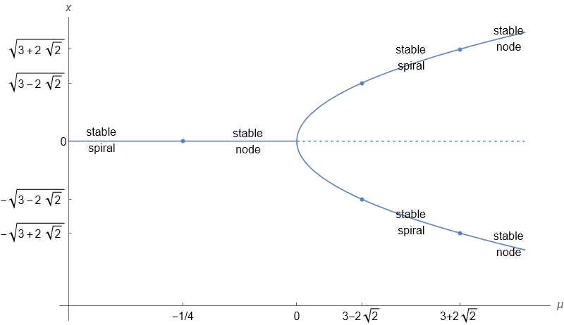
At \(\mu=0\) the stable equilibrium at \(x=0\) becomes unstable and from it emerges two stable equilibria. This type of bifurcation is called a “pitchfork bifurcation”.

Bifurcation

A bifurcation of an equilibrium point is a change in the number or stability of equilibrium points in a differential equation as a parameter changes its value.

24.3. Classifying bifurcations¶

In this subsection we will look at some of the most commonly encountered types of bifurcation. The example systems used to illustrate feature only a single dependent variable, so we do not need to use the Jacobian to classify. We can simply consider the direction of the change vectors either side of any equilibrium points, as we did in Section 22.1.

24.3.1. Pitchfork bifurcation¶

A pitchfork bifurcation occurs when a system transitions from one equilibrium point to three.

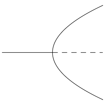
In a supercritical pitchfork bifurcation a stable equilibrium turns unstable and two stable equilibria emerge either side
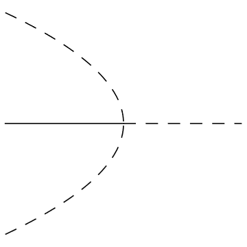
In a subcritical pitchfork bifurcation an unstable equilibrium turns stable and two unstable equilibria emerge either side.

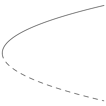
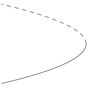
Illustrations of both types are shown below. In these examples the parameter \(\mu\) is shown on the horizontal axis and the equilibrium point is shown on the vertical axis.

Terminology

Note that subcritical and supercritical describe the stability of the equilibrium points and are not dependent on which direction the pitchfork faces.

Supercritical case

\[\begin{equation*} \dot{x}=\mu x -x^3 \end{equation*}\]

Subcritical case

\[\begin{equation*} \dot{x}=\mu x +x^3 \end{equation*}\]

Exercise 24.2

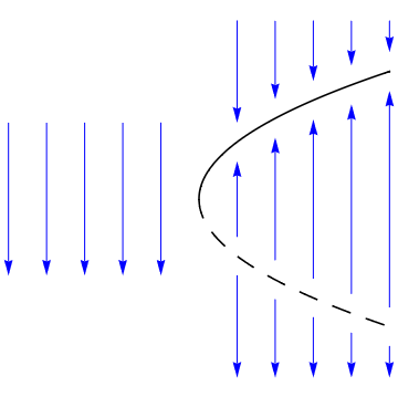
Pick one of the two examples above and sketch change vectors on the diagram. Note that in the bifurcation diagram the \(x\) axis is vertical, so the change vectors will point either up or down depending on the sign of \(\dot{x}\)

Solution:

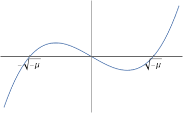
The plot below is for the case \(\dot{x}=\mu x +x^3\)

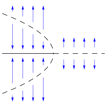
For example, consider that for \(\mu<0\) the shape of the change function is as shown below. The change function is positive for \(-\sqrt{\mu}<x<0\), negative for \(x<-\sqrt{\mu}\), etc.

Classification using the 1D Jacobian

It is also possible to classify the stability of these equilibria using the 1D Jacobian. For a problem

(24.11)¶\[\begin{equation} \dot{x} = f(x) \end{equation}\]

the Jacobian is simply \(f^{\prime}(x)\). If \(x_0\) is an equilibrium point then \(f^{\prime}(x_0)\) determines whether the stability as follows:

If \(f^{\prime}(x_0)>0\) the equilibrium point is unstable,
If \(f^{\prime}(x_0)<0\) the equilibrium point is stable.

Can you understand why this is so? Think about the shape of the plot \(f(x)\), which determines the direction vectors \(\dot{x}\).

Exercise 24.3

Use the 1D Jacobian to verify the stability results for the case where \(f(x)=\mu x+x^3\).

Solution:

We have \(f^{\prime}(x)=\mu+ 3x^2\) and so

\(f^{\prime}(0)=\mu\)
\(f^{\prime}(\pm\sqrt{-\mu})=-2\mu\)

This concludes that :

the equilibrium point \(x=0\) is stable for \(\mu<0\) and unstable for \(\mu>0\),
the equilibrium points \(x=\pm\sqrt{-\mu}\) are unstable where they exist.

The results are consistent with what we found by sketching.

24.3.2. Saddle node bifurcation¶

A saddle node bifurcation or fold bifurcation occurs when two equilibrium points coalesce and annihilate each other. The supercritical and subcritical cases are shown below.

Supercritical case

\[\begin{equation*} \dot{x} = \mu -x^2 \end{equation*}\]

Subcritical case

\[\begin{equation*} \dot{x} = \mu +x^2 \end{equation*}\]

Exercise 24.4

Pick one of these two cases and plot the change vectors on the diagram. Also use the 1D Jacobian to verify your results.

For the case where \(f(x)=\mu-x^2\) the equilibria are at \(x=\pm\sqrt{\mu}\), \(\mu>0\).

\(f^{\prime}(\sqrt{\mu})=-2\mu\) : stable
\(f^{\prime}(-\sqrt{\mu})=2\mu\) : unstable

The diagram is shown below.

Exercise 24.5

Show that the following two-dimensional problem has a saddle-node bifurcation at \(\mu=0\):

\[\begin{align*} \dot{x}&=\mu-x^2\\ \dot{y}&=-y \end{align*}\]

Solution

Equilibrium points \((\pm\sqrt{\mu},0)\), for \(\mu\geq 0\)

Jacobian: \(\begin{bmatrix}-2x & 0\\0&-1\end{bmatrix}\)

Eigenvalues: \(\lambda=-1,\mp2\sqrt{\mu}\)

The point \((0,-\sqrt{\mu})\) is a saddle node

The point \((0,\sqrt{\mu})\) is a stable node

24.3.3. Transcritical bifurcation¶

A transcritical bifurcation is characterised by a system with one stable equilibrium point and one unstable equilibrium point, which exchange stability when they collide. An example of a transcritical bifurcation is illustrated below.

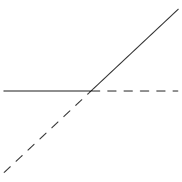
(24.12)¶\[\begin{equation} \dot{x}=\mu x - x^2 \end{equation}\]

The equilibrium points are at \(x=0\) and \(x=\mu\). To classify their stablity, either use the change vectors or simply note that for \(f(x)=\mu x - x^2\) we have

\(f^{\prime}(0)=\mu\) : stable for \(\mu<0\)
\(f^{\prime}(\mu)=-\mu\) : stable for \(\mu>0\)

Mathematics for Natural Sciences 2

Bifurcation analysis

Contents