10. Vector Calculus Theorems¶

Although the ideas in vector calculus seem quite distinct, area, surface and volume integrals as well as the gradient, divergence and curl, it turns out that they are connected together thanks to a couple of quite important theorems. These can in some cases simplify a calculation that we are aiming to do and/or give us a better intution about a system.

10.1. (Gauss-)Divergence Theorem¶

Lets think about a closed surface \(S\) in a space, this surface area therefore encloses a volume \(V\), i.e. it forms the boundary \(S = \partial V\) (not to be confused with taking some partial derivative!), as depicted in Fig. 10.1.

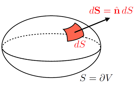
Fig. 10.1 Vectorial surface-area element \(\mathrm{d}{\bf S}\) of a closed surface \(S = \partial V\), with the convention that \(\mathrm{d}{\bf S} = \hat{\bf b} \mathrm{D}S\) points outwards.¶

Thinking about a vector field \({\bf G}({\bf r})\) through the closed surface \(S\), one thing we can do is count the flux from the surface intregral:

\[\int_S {\bf G}({\bf r})\cdot \mathrm{d}{\bf S}\]

We can see that if the field is uniform, say \(\nabla \cdot {\bf G} = 0\), then this net flux will zero (all incoming vectors = all out going vectors), however if there is a divergence in the enclosed volume \(\nabla \cdot {\bf G} \neq 0\), then there would be a net flux through the surface (with the sign of the flux being related to the sign ofthe divergence).
This result gives us the Divergence Theorem:

\[\int_S {\bf G}({\bf r})\cdot \mathrm{d}{\bf S} = \int_V \left(\nabla \cdot G\right)\,\mathrm{d}V\]

10.1.1. Divergence Theorem Example¶

Lets start with an example, for the vector field:

\[\begin{split}{\bf G}({\bf r}) = \begin{pmatrix} x^2 \\ y \\ z \end{pmatrix}\end{split}\]

over a cubic volume, centered on the origin, with corners \((\pm 1,\, \pm 1,\, \pm 1)\), as depicted in Fig. 10.2

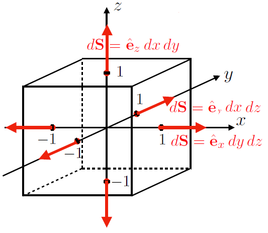
Fig. 10.2 An example cubic surface around some vector field divergence.¶

If we compute the surface integral:

\[\begin{split}I = \int_{S = \partial V} {\bf G}({\bf r})\cdot \mathrm{d}{\bf S} &=& \, \int_{-1}^1 \,\mathrm{d}y\,\int_{-1}^1\,\mathrm{d}z \,\begin{pmatrix} 1 \\ y \\ z \end{pmatrix} \cdot \begin{pmatrix} 1 \\ 0 \\ 0 \end{pmatrix} + \int_{-1}^1 \,\mathrm{d}y\,\int_{-1}^1\,\mathrm{d}z \,\begin{pmatrix} 1 \\ y \\ z \end{pmatrix} \cdot \begin{pmatrix} - \\ 0\\ 0 \end{pmatrix} \\ &+& \, \int_{-1}^1 \,\mathrm{d}x\,\int_{-1}^1\,\mathrm{d}z \,\begin{pmatrix} x^2 \\ 1 \\ z \end{pmatrix} \cdot \begin{pmatrix} x^2 \\ 1 \\ 0 \end{pmatrix} + \int_{-1}^1 \,\mathrm{d}y\,\int_{-1}^1\,\mathrm{d}z \,\begin{pmatrix} x^2 \\ -1 \\ z \end{pmatrix} \cdot \begin{pmatrix} x^2 \\ -1 \\ 0 \end{pmatrix} \\ &+& \, \int_{-1}^1 \,\mathrm{d}x\,\int_{-1}^1\,\mathrm{d}y \,\begin{pmatrix} x^2 \\ y \\ 1 \end{pmatrix} \cdot \begin{pmatrix} x^2 \\ y \\ 1 \end{pmatrix} + \int_{-1}^1 \,\mathrm{d}x\,\int_{-1}^1\,\mathrm{d}y \,\begin{pmatrix} x^2 \\ y \\ -1 \end{pmatrix} \cdot \begin{pmatrix} x^2 \\ y \\ -1 \end{pmatrix} \\ &=& \, 2 \int_{-1}^1 \,\mathrm{d}x\,\int_{-1}^1\,\mathrm{d}z + \int_{-1}^1 \,\mathrm{d}x\,\int_{-1}^1\,\mathrm{d}y = 16\end{split}\]

A little long! However using the Gauss’s divergence theorem:

\[\begin{split}\nabla \cdot {\bf G} &= 2x + 2\\ I &= \int_{V} (\nabla \cdot {\bf G})\,\mathrm{d}V = \int_{-1}^1\,\mathrm{d}x\, \int_{-1}^1\,\mathrm{d}y\, \int_{-1}^1\,\mathrm{d}z (2x + 2)\\ &= 4\int_{-1}^1\,(2x+2)\,\mathrm{d}x = 4\Bigg[x^2 + 2x\Bigg]_{-1}^1 = 16\end{split}\]

In agreement with the previous result and whole lot easier to do!

10.1.2. A Sketch of a Proof¶

We can sketch out a proof of this result, using the same set up as previously, as seen in Fig. 10.3,

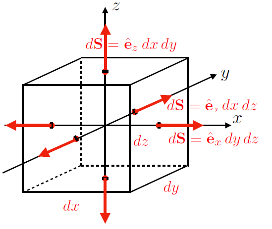
Fig. 10.3 An infinitesimal cubic surface \(\mathrm{d}V = \mathrm{d}x\,\mathrm{d}y\,\mathrm{d}z\) around some vector field divergence.¶

Thinking about an infinitesimal flux element \(\mathrm{d}F\) for a vector field \({\bf G}({\bf r})\) crossing the sides of the infinitesimal volume element \(\mathrm{d}V = \mathrm{d}x\,\mathrm{d}y\,\mathrm{d}z\):

(10.1)¶\[\begin{split}\mathrm{d}F &= {\bf G}\left({\bf r} + \frac{1}{2}\mathrm{d}x\,\hat{\bf x} \right)\cdot \hat{\bf x}\,\mathrm{d}y\,\mathrm{d}z + {\bf G}\left({\bf r} - \frac{1}{2}\mathrm{d}x\,\hat{\bf x} \right)\cdot (-\hat{\bf x})\,\mathrm{d}y\,\mathrm{d}z\\ &+&\, {\bf G}\left({\bf r} + \frac{1}{2}\mathrm{d}y\,\hat{\bf y} \right)\cdot \hat{\bf y}\,\mathrm{d}x\,\mathrm{d}z + {\bf G}\left({\bf r} - \frac{1}{2}\mathrm{d}x\,\hat{\bf y} \right)\cdot (-\hat{\bf y})\,\mathrm{d}x\,\mathrm{d}z\\ &+&\, {\bf G}\left({\bf r} + \frac{1}{2}\mathrm{d}z\,\hat{\bf z} \right)\cdot \hat{\bf z}\,\mathrm{d}x\,\mathrm{d}y + {\bf G}\left({\bf r} - \frac{1}{2}\mathrm{d}x\,\hat{\bf z} \right)\cdot (-\hat{\bf z})\,\mathrm{d}x\,\mathrm{d}y\end{split}\]

The first line of (10.1) reduces to:

\[\begin{split}&&\, \left[{\bf G}\left({\bf r} + \frac{1}{2}\mathrm{d}x\,\hat{\bf x} \right)\cdot \hat{\bf x} + {\bf G}\left({\bf r} - \frac{1}{2}\mathrm{d}x\,\hat{\bf x} \right)\cdot (-\hat{\bf x})\right]\,\mathrm{d}y\,\mathrm{d}z\\ &= \left[G_x\left({\bf r} + \frac{1}{2}\mathrm{d}x\,\hat{\bf x} \right) - G_x\left({\bf r} - \frac{1}{2}\mathrm{d}x\,\hat{\bf x} \right)\right]\,\mathrm{d}y\,\mathrm{d}z\\\end{split}\]

If we do a Taylor expansion of each vector field, around \(G_x({\bf r})\):

\[\begin{split}&= \left[G_x({\bf r}) + \frac{1}{2}\partial_x G_x({\bf r})\,\mathrm{d}x - \left(G_x({\bf r}) - \frac{1}{2}\partial_x G_x({\bf r})\,\mathrm{d}x \right)\right]\,\mathrm{d}y\,\mathrm{d}z\\ &= \partial_x G_x \,\mathrm{d}x\,\mathrm{d}y\,\mathrm{d}z\end{split}\]

We can do similar for the second and third lines of (10.1) to find the result:

And through suitable coordinate transforms we could prove this result for any coordinate system. Hence the flux across the cubes sides is related to the divergence of the vector field over the volume element.

If we then proceed with integrating this flux over the over a given volume, then we can think of this as summing up little cubes with volume \(\mathrm{d}V\), as depicted in Fig. 10.4.

Fig. 10.4 Infinitesimal cubic volume \(\mathrm{d}V = \mathrm{d}x\,\mathrm{d}y\,\mathrm{d}z\) making up some volume \(V\).¶

This means we are summing up neighbouring cubes, where the outgoing flux \(\int \,\mathrm{d}F > 0\) from one will be an incoming flux \(\int \,\mathrm{d}F < 0\) for another cube, as depicted in Fig. 10.5.

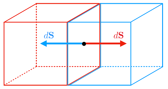
Fig. 10.5 A schematic of the infinitesimal flux contributions from neighbouring infintesimal cubic volumes.¶

Therefore we see that the only remaining contributions to the summing of the fluxes over the volume will be from the volumes surface, hence:

\[\int_V\,\mathrm{d}F = \int_{S = \partial V}\,\mathrm{d}F = \iint_{S = \partial V}\,{\bf G}({\bf r})\cdot \mathrm{d}{\bf S} = \iiint \Bigg( \nabla \cdot {\bf G}({\bf r})\Bigg)\,\mathrm{d}V\]

which is the desired result.

10.2. (Kelvin-)Stoke’s Theorem¶

Stokes’s theorem states that the loop integral of a vector field \({\bf G}({\bf r})\) around the boundary \(C = \partial S\) of an open surface \(S\) is equal to the flux of the curl of the vector field, \(\nabla \times {\bf G}({\bf r})\) through the surface;

\[\oint_{C = \partial S} {\bf G}({\bf r}) \cdot \mathrm{d}{\bf r} = \iint_{S} \Bigg(\nabla \times {\bf G}\Bigg)\cdot\mathrm{d}{\bf S}\]

where the orientation of this closed contour is given by the right hand rule, as depicted in Fig. 10.6:

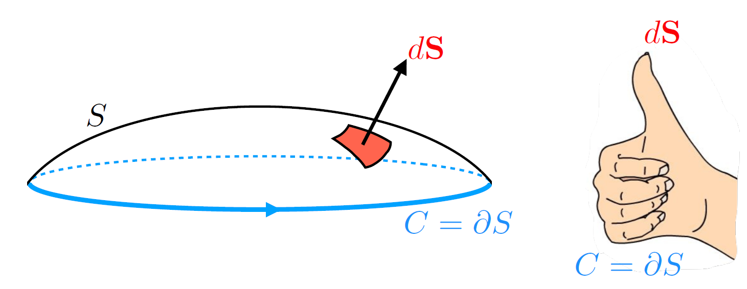
Fig. 10.6 The relevant orientation of the closed contour used in Stoke’s theorem.¶

10.2.1. Stoke’s Theorem Example¶

Lets look at an example, with the vector field \({\bf G}({\bf r}) = \begin{pmatrix} y \\ -z \\ -x^2 \end{pmatrix}\) over a closed path around a circular arc around the origin, which we depict in Fig. 10.7:

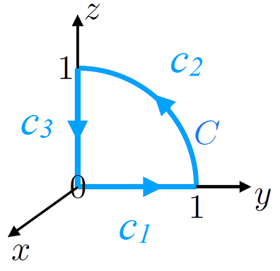
Fig. 10.7 Closed contour around the origin - note that this contour bounds an area that is the quarter of a unit circle centered on the origin.¶

The parameterisation of the line integral will not change its result (nor should the starting point for a loop integral), so we will start at the origin and parameterise the three sections of the contour \(C_1,\,C_2,\, C_3\) using \(t\), with \(t \in [0,\,1]\) along each piece:

\[\begin{split}C_1: {\bf r}(t) &= \begin{pmatrix} 0 \\ t \\ 0 \end{pmatrix} \Rightarrow {\bf G}({\bf r}) = \begin{pmatrix} t \\ 0 \\ 0 \end{pmatrix}, \quad {\bf r'}(t) = \begin{pmatrix} 1 \\ 0 \\ 0 \end{pmatrix}\\ C_2: {\bf r}(t) &= \begin{pmatrix} 0 \\ \cos(\pi t/2) \\ \sin(\pi t/2) \end{pmatrix} \Rightarrow {\bf G}({\bf r}) = \begin{pmatrix} \cos(\pi t/2) \\ -\sin(\pi t/2) \\ 0 \end{pmatrix}, \quad {\bf r'}(t) = \begin{pmatrix} 0 \\ -\frac{\pi}{2}\sin(\pi t/2) \\ \frac{\pi}{2}\cos(\pi t/2) \end{pmatrix}\\ C_3: {\bf r}(t) &= \begin{pmatrix} 0 \\ 0 \\ 1-t \end{pmatrix} \Rightarrow {\bf G}({\bf r}) = \begin{pmatrix} 0 \\ -(1-t) \\ 0 \end{pmatrix}, \quad {\bf r'}(t) = \begin{pmatrix} 0 \\ 0 \\ -1 \end{pmatrix}\end{split}\]

Therefore we can calculate the line integral:

\[\begin{split}I &= \int_C {\bf G}({\bf r})\cdot \mathrm{d}{\bf r} = \int_0^1 {\bf G}({\bf r})\cdot {\bf r'}\,\mathrm{d}t\\ &= \int_0^1 \begin{pmatrix} t \\ 0 \\ 0 \end{pmatrix} \cdot \begin{pmatrix} 0 \\ 1 \\ 0 \end{pmatrix}\,\mathrm{d}t + \int_0^1 \begin{pmatrix} \cos(\pi t/2) \\ -\sin(\pi t/2) \\ 0 \end{pmatrix}\cdot \begin{pmatrix} 0 \\ -\frac{\pi}{2}\sin(\pi t/2) \\ \frac{\pi}{2}\cos(\pi t/2) \end{pmatrix}\,\mathrm{d}t + \int_0^1 \begin{pmatrix} 0 \\ -(1-t) \\ 0 \end{pmatrix} \cdot\begin{pmatrix} 0 \\ 0 \\ -1 \end{pmatrix}\,\mathrm{d}t\\ &= \frac{\pi}{2}\int_0^1\sin^2(\pi t/2)\,\mathrm{d}t = \frac{\pi}{4}\int_0^1\Bigg (1-\cos(\pi t)\Bigg)\,\mathrm{d}t = \frac{\pi}{4}\Bigg[t - \frac{1}{\pi}\sin(\pi t)\Bigg]_0^1 =\frac{\pi}{4}\end{split}\]

Using Stoke’s theorem, we are free to find formally any surface which would be bounded by the contour - however clearly the easiest to work with is the area of the quarter circle, sitting on the \(y-z\) plane. To make sure the orientation of the contour matches with the right hand rule, we have \(\mathrm{d}{\bf S} = \mathrm{d}y\,\mathrm{d}z\,\hat{\bf x}\), therefore given that

\[\begin{split}\nabla \times {\bf G} = \begin{pmatrix} 1\\ 2x\\ -1\end{pmatrix}\end{split}\]

we can find:

\[\begin{split}I &= \iint_S\Bigg( \nabla \times {\bf G}\Bigg)\cdot\mathrm{d}{\bf S} \\ I &= \iint_S \begin{pmatrix} 1\\ 2x\\ -1\end{pmatrix}\cdot \begin{pmatrix} 1\\ 0\\ 0\end{pmatrix}\,\mathrm{d}y\,\mathrm{d}z\\ &= \iint_S \,\mathrm{d}y\,\mathrm{d}z = \frac{1}{4}\pi 1^2 = \frac{\pi}{4}\end{split}\]

Therefore for quite a lot less work, we find the same result!

10.2.2. A Sketch of a Proof¶

Lets consider a vectorial surface area element \(\mathrm{d}{\bf S} = \mathrm{d}x\,\mathrm{d}y\,\hat{\bf z}\), as depicted in Fig. 10.8:

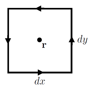
Fig. 10.8 Closed infinitesimal contour around some point \({\bf r}\).¶

We can therefore find the loop integral of a vector field \({\bf G}({\bf r})\) around this contour as:

\[\begin{split}dI &= {\bf G}\left({\bf r} - \frac{1}{2}\mathrm{d}y\,\hat{\bf y} \right)\cdot \hat{\bf x}\,\mathrm{d}x + {\bf G}\left({\bf r} + \frac{1}{2}\mathrm{d}x\,\hat{\bf x} \right)\cdot \hat{\bf y}\,\mathrm{d}y \\ &+&\, {\bf G}\left({\bf r} + \frac{1}{2}\mathrm{d}y\,\hat{\bf y} \right)\cdot (-\hat{\bf x})\,\mathrm{d}x + {\bf G}\left({\bf r} + \frac{1}{2}\mathrm{d}x\,\hat{\bf x} \right)\cdot (-\hat{\bf y})\,\mathrm{d}y \\ &= \left[G_x \left({\bf r} - \frac{1}{2}\mathrm{d}y\,\hat{\bf y} \right) - G_x\left({\bf r} + \frac{1}{2}\mathrm{d}y\,\hat{\bf y} \right) \right]\,\mathrm{d}x + \left[ G_y\left({\bf r} + \frac{1}{2}\mathrm{d}x\,\hat{\bf x} \right) - G_y\left({\bf r} - \frac{1}{2}\mathrm{d}x\,\hat{\bf x} \right)\right]\,\mathrm{d}y\end{split}\]

Taking a Taylor expansion around \({\bf G}({\bf r})\), we find:

\[\begin{split}&= -\partial_y G_x({\bf r})\,\mathrm{d}x\,\mathrm{d}y + \partial_x G_y({\bf r})\,\mathrm{d}x\,\mathrm{d}y \\ &= \Bigg(\nabla \times {\bf G}\Bigg)_z\,\mathrm{d}x\,\mathrm{d}y = \Bigg(\nabla \times {\bf G}\Bigg)\cdot \hat{\bf z}\,\mathrm{d}x\,\mathrm{d}y\\ &= \Bigg(\nabla \times {\bf G}\Bigg)\cdot\mathrm{d}{\bf S}\end{split}\]

Which if we integrate up, we find \(I = \iint_S (\nabla \times {\bf G})\cdot \mathrm{d}{\bf S}\). Thinking carefully these loop integrals however, if we sum up infinitesimal areas (plaquettes if you will), then along the surface neighbouring areas will have cancellation occuring, as depicted in Fig. 10.9:

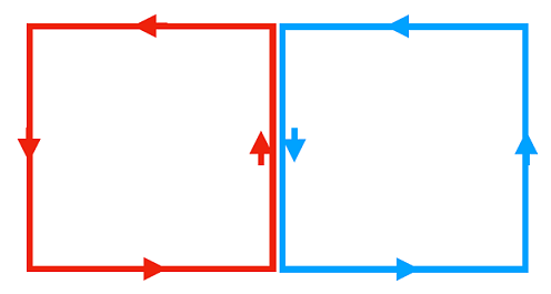
Fig. 10.9 Neighbouring infinitesimal contours along some surface, we find that there will be a net cancellation occuring along shared sides.¶

This means that the only interbal contributions to summing up these loop integrals will be those along the boundary, hence:

\[\int_S\,\mathrm{d}I = \int_{C=\partial S}{\bf G}\cdot \mathrm{d}{\bf r} = \iint_S (\nabla \times {\bf G})\cdot \mathrm{d}{\bf S}\]