Linear Transformations
Contents
17. Linear Transformations
In this section we learn to understand matrices geometrically as functions, or transformations. We briefly discuss transformations in general, then specialize to matrix transformations, which are transformations that come from matrices.
17.1. Linear Transformations
A function is a rule that takes inputs and transforms them to outputs. For example, a function \(f:\mathbb{R}\rightarrow\mathbb{R}\),
is a function that takes a real number \(x\) as input and outputs another real number, the square of the input. On the other hand, the function \(g:\mathbb{R}^2\rightarrow \mathbb{R}\),
is a function which maps 2-dimensional vectors \((x, y) \in \mathbb{R}^2\) to real numbers.
Functions can also be defined geometrically. For example, the following are valid function definitions:
\(R_\theta:\mathbb{R}^2\rightarrow\mathbb{R}^2\) corresponding to a \(\theta\) anticlockwise rotation around the origin.
\(U:\mathbb{R}^2\rightarrow\mathbb{R}^2\) corresponding to a translation by the vector \(\begin{pmatrix}1\\-1\end{pmatrix}\).
Definition
Suppose \(f:\mathbb{R}^n \rightarrow \mathbb{R}^m\) is a function such that
and
for all \(u, v \in\mathbb{R}^n\) and \(a\in\mathbb{R}\).
Then \(f\) is a linear transformation.
Attention
In mathematics, the words function, map and transformation can be used interchangeably. So ‘linear function’, ‘linear map’ and ‘linear transformation’ all have the same meaning.
In practice, we often prefer the word ‘transformation’ when we want to emphasise the geometrical nature of a function.
You can think of this definition as the transformation of any linear combination of vectors is the same as the linear combination of the transformed vectors.
Rotation is an example of a linear transformation:
We can add vectors \(u\) and \(v\) and then rotate, or we can rotate \(u\) and \(v\) and then add, as illustrated in Fig. 17.1.
We can scale \(u\) and then rotate, or we can rotate \(u\) and then scale.
Fig. 17.1 The parallelogram rule for vector addition shows that \(R_\theta(u + v) = R_\theta(u) + R_\theta(v)\).
Properties of Linear transformations
If \(T:\mathbb{R}^n \rightarrow \mathbb{R}^m\) is a linear transformation, then
and for any vectors \(v_1,\ldots,v_k \in \mathbb{R}^n\) and scalars \(a_1,\ldots a_k \in \mathbb{R}\)
The first property \(T(0)=0\) follows from the second part of the definition of linearity. Note that here \(0\) represents a vector and we geometrically we can think of this as saying that a linear transformation takes the origin to the origin.
Example
1. A non-linear transformation
The transformation \(T:\mathbb{R} \rightarrow \mathbb{R}\) defined by \(T(x) = x + 1\) is not a linear transformation.
We can easily prove this by showing that \(T\) fails to fix the origin:
Therefore \(T\) is not a linear transformation, even though the graph of \(T(x)\) is a straight line.
2. A linear transformation
Suppose \(U:\mathbb{R}^2 \rightarrow \mathbb{R}^2\) be defined by \(U(x) = 2x\).
\(U\) is a dilation which doubles the size of every vector. We show that this is a linear transformation by checking the definition. Let \(u, v \in \mathbb{R}^2\) and \(a \in \mathbb{R}\). Then
and
Exercise 17.1
Which of the following functions are linear transformations?
1. \(T:\mathbb{R}^2\rightarrow\mathbb{R}^2\),
2. \(f:\mathbb{R}\rightarrow\mathbb{R}\),
3. \(U:\mathbb{R}^3\rightarrow\mathbb{R}^2\),
17.2. Matrix Transformations
Now let \(A\) be an \((m \times n)\) matrix. Then \(A\) defines a function
where
In other words, \(A\) defines a function which takes a vector \(x \in \mathbb{R}^n\) and transforms it to a vector \(Ax \in \mathbb{R}^m\). In fact, it turns out that the function defined by multiplication by a matrix is a linear transformation.
Theorem
If \(A\) is an \((m \times n)\) matrix \(A\) then the function
defined by
is a linear transformation which takes the vector \(x \in \mathbb{R}^n\) to the vector \(Ax \in \mathbb{R}^m\).
The proof of this follows directly from the definitions of matrix arithmetic:
There is essentially nothing new here, beyond the notation and a slightly different way of thinking about matrix multiplication. In the next section we will see how thinking of a matrix as a transformation allows us to picture its effect geometrically.
17.3. Geometrical Interpretation of Matrices
Consider the matrix
which defines the linear transformation \(T:\mathbb{R}^2 \rightarrow \mathbb{R}^2\) defined by \(T(x) = Ax\).
Given a vector \(x=\begin{pmatrix}x_1\\x_2\end{pmatrix}\) we can consider the effect of the transformation \(T\):
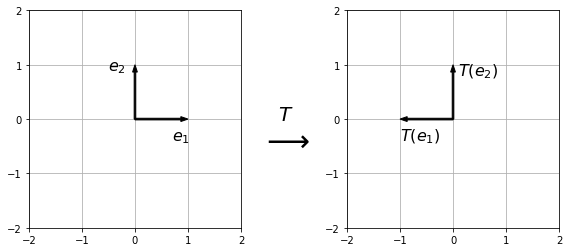
Multiplication by \(A\) negates the \(x_1\) co-ordinate and leaves the \(x_2\) co-ordinate unchanged i.e. it reflects over the \(x_2\) axis.
We can illustrate this by picturing the effect of the transformation on the unit co-ordinate vectors \(e_1 = \begin{pmatrix}1\\0\end{pmatrix}\) and \(e_2=\begin{pmatrix}0\\1\end{pmatrix}\):
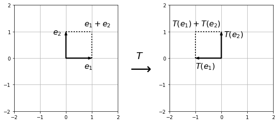
Furthermore, once we know the transformed unit vectors, we can use the linearity of the transformation to determine how any vector is transformed. Given a vector \(x = \begin{pmatrix}x_1\\x_2\end{pmatrix}\), we can write \(x\) as a sum of unit co-ordinate vectors:
and use the linearity property to calculate the result
For example, the vector \(e_1 + e_2\) is transformed to \(T(e_1) + T(e_2)\) so we can use this to draw the image of the unit square which has vertices \(0\), \(e_1\), \(e_2\) and \(e_1 + e_2\):
Example
Determine the geometrical effect of the transformation given by the matrix
Solution
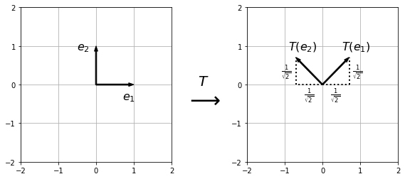
\(A\) represent a rotation anticlockwise by \(\pi/4\).
Exercise 17.2
Describe the geometrical effect of the following matrices:
1. \(A = \begin{pmatrix}\frac{1}{\sqrt{2}}&\frac{1}{\sqrt{2}}\\\frac{1}{\sqrt{2}}&\frac{1}{\sqrt{2}}\end{pmatrix}\)
2. \(B = \begin{pmatrix}k & 0\\0 & 1\end{pmatrix}\)
3. \(C = \begin{pmatrix}1 & k\\0 & 1\end{pmatrix}\)
17.4. The Matrix of a Linear Transformation
In this section will learn that all linear transformations are matrix transformations - in other words, any function \(T\) which satisfies the linearity properties can be written as a matrix \(T(x) = Ax\). Before doing so, we need the following important notation.
Definition
The standard coordinate vectors in \(\mathbb{R}^n\) are the \(n\) vectors
The standard coordinate vectors are useful because of the following property:
Multiplying a matrix by the standard co-ordinate vector \(e_i\) selects the \(i\)th column of the matrix.
Suppose that an \((m \times n)\) matrix \(A\) is composed of the \(n\) column vectors \(v_1, v_2, \ldots, v_n\). Then,
For example,
Theorem
Let \(T:\mathbb{R}^n \rightarrow \mathbb{R}^m\) be a linear transformation. Then the \((m \times n)\) matrix
is the matrix corresponding to the transformation \(T\) and \(T(x)=Ax\).
Using this theorem, we can write down the matrix of any linear transformation.
Example
Determine the matrix of the linear transformation \(T:\mathbb{R}^2 \rightarrow \mathbb{R}^2\) corresponding to reflection across the line \(x_2 = -x_1\).
Solution
First, determine the transformation of the unit coordinate vectors.
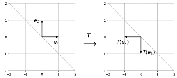
Therefore the matrix,
is the matrix of the transformation \(T\).
Exercise 17.3
1. Find the transformation of the basis vectors under reflection in the line \(y=kx, k\in\mathbb{R}\), giving your answer in terms of the angle between the line and the \(x\)-axis. Hence, find the image of the triangle with vertices \((1,3)\), \((3,1)\), \((2,2)\) under reflection in the line \(y=\sqrt{3}x\).
2. Sketch the image of the unit square with vertices \((0,0)\), \((0,1)\), \((1,0)\), \((1,1)\) under the linear transform \(\left(\begin{array}{cc}1 & 0 \\3 & 1 \\\end{array}\right)\). Try to describe this transformation in words.
17.5. Rotation matrices in 2D
Suppose the linear transformation \(T:\mathbb{R}^2 \rightarrow \mathbb{R}^2\) corresponds to an anticlockwise rotation by an angle \(\theta\) around the origin. Then we can use trigonometry to determine the destination of the coordinate vectors under \(T\):
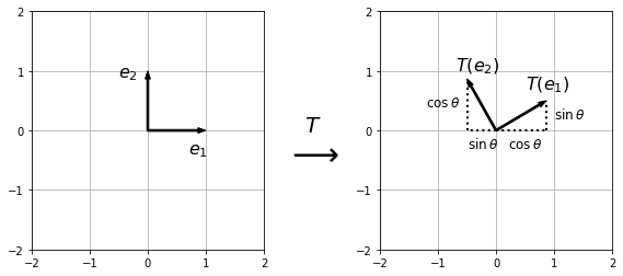
Rotation Matrix
The matrix corresponding to an anticlockwise rotation by \(\theta\) degrees around the origin is given by:
17.6. The identity matrix
The identity matrix \(I_n\) is the unique \((n \times n)\) matrix which has the property
for any \(x \in \mathbb{R}^n\).
The identity matrix transforms the vector \(x\) to itself. It plays the same role in matrix multiplication as the number 1 does for multiplication of real numbers.
Definition
The identity matrix
We usually drop the subscript \(n\) when working with the identity matrix, because the order can be inferred.
Exercise 17.4
Calculate \(I\begin{pmatrix}1 & 2\\3 & 4\end{pmatrix}\) and \(\begin{pmatrix}1 & 2\\3 & 4\end{pmatrix}I\).
Use the identify matrix to factorise \(AB+\lambda B\) where \(\lambda\) is a scalar and \(A,B\) are square matrices.
17.7. Composition of Linear Transformations
Given two linear transformations \(T:\mathbb{R}^n\rightarrow\mathbb{R}^m\) and \(U:\mathbb{R}^p\rightarrow\mathbb{R}^n\), the function \(T \circ U:\mathbb{R}^p\rightarrow\mathbb{R}^m\) is the composition of the two functions. That is, the function corresponding to applying first the function \(U\), then the function \(T\).
If \(T\) and \(U\) are linear transformations with matrices \(A\) and \(B\) respectively, then the product matrix \(AB\) represents the composition function \((T\circ U)\).
For example, suppose matrices \(A\) and \(B\) represent reflection in the \(y\)- and \(x\)-axis respectively:
Then the matrix \(AB\) represents a rotation by \(\pi\) around the origin:
Example
In Exercise 17.3 we reflected a set of points in the line through the origin at angle \(\theta\) with the \(x\)-axis. An equivalent way to do this would be to rotate clockwise by angle \(\theta\), reflect in the line \(y=0\) and then rotate back!
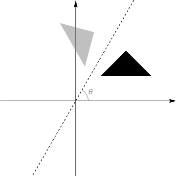
Fig. 17.2 Reflection in a line as a three-step process. Equivalent to a reflection in the dashed line, we can 1) rotate clockwise by angle \(\theta\) 2) reflect in the horizontal axis 3) rotate anti-clockwise by angle \(\theta\).
The transformation matrix for reflection in the line \(y=0\) is just \(\left(\begin{array}{cc}1 & 0 \\0 & -1 \\\end{array}\right)\), since \(x\mapsto x \), \(y\mapsto -y\).
Therefore, in matrix terms, we have
which is the result given previously.
Exercise 17.5
Use a composition of three matrix transformations to calculate the 2-d transformation matrix for a stretch, scale factor \(k\) parallel to the line \(y=\tan(\theta)x\).
17.8. Solutions
1. and 2. Non-linear.
3. Linear.
1. \(A = \begin{pmatrix}\frac{1}{\sqrt{2}}&\frac{1}{\sqrt{2}}\\\frac{1}{\sqrt{2}}&\frac{1}{\sqrt{2}}\end{pmatrix}\)
\(A\) projects vectors onto the line \(y=x\).
2. \(B = \begin{pmatrix}k & 0\\0 & 1\end{pmatrix}\)
\(B\) stretches vectors parallel to the \(x\)-axis by a scale factor \(k\).
3. \(C = \begin{pmatrix}1 & k\\0 & 1\end{pmatrix}\)
\(C\) represents a vertical shear by a factor \(k\).
1. The transformation of the basis vectors, shown in the graphic below is:
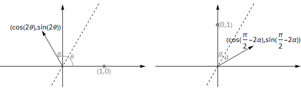
Fig. 17.3 reflection of basis vectors in the line \(y=\mathrm{tan}(\theta)x\).
and so the transformation matrix is \(T=\left(\begin{array}{cc}\cos 2\theta & \sin 2\theta \\ \sin 2\theta & -\cos 2 \theta \end{array}\right)\)
For the line \(y=\sqrt{3}x\) we have \(\theta=\frac{\pi}{3}\), so \(T=\left(\begin{array}{cc}\cos(2\frac{\pi}{3})&\sin(2\frac{\pi}{3})\\\sin(2\frac{\pi}{3})&-\cos(2\frac{\pi}{3})\end{array}\right)=\frac{1}{2}\left(\begin{array}{cc}-1 & \sqrt{3} \\\sqrt{3} & 1 \\\end{array}\right)\).
The transformation of the given points is
A plot of the reflection is shown below.
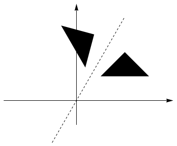
Fig. 17.4 reflected triangle.
2.
The image below shows the unit square under the transform \(\left(\begin{array}{cc}1&0\\k&1\end{array}\right)\) as the constant \(k\) is adjusted between 0 and 3.
Fig. 17.5 vertical shear.
Note that we can write this transform as \(\left(\begin{array}{cc}1 & 0 \\0 & 1 \\\end{array}\right)+\left(\begin{array}{cc}0 & 0 \\k & 0 \\\end{array}\right)\).
The first term is just the identity matrix that maps points to themselves, and the second term transforms the y coordinate of each point by an amount proportional to the \(x\) coordinate, so points that are further from the \(y\)-axis are stretched more. This type of transform is known as a vertical shear.
We can achieve the same effect parallel to the horizontal axis by taking the transform (known as horizontal shear by taking the transform \(\left(\begin{array}{cc}1&k\\0&1\end{array}\right)\).
\(I\begin{pmatrix}1 & 2\\3 & 4\end{pmatrix}=\begin{pmatrix}1 & 2\\3 & 4\end{pmatrix}I = \begin{pmatrix}1 & 2\\3 & 4\end{pmatrix}\).
\(AB+\lambda B = (A+\lambda I)B\).
We can describe this transformation as a rotation by \(\theta\) followed by a scale 2 stretch parallel to the \(x\)-axis followed by a rotation by \(-\theta\).