1. Multivariable Calculus¶

1.1. First Partial Derivatives¶

The plot shown in Fig. 1.1 is of a function, $f(x,\, y)= x^3 - y^3 - 2xy + 2$, on which curves marked on the surface for lines of constant $x,\,y$.

We can consider the rate of change of the function, however since it is a function of two variables, we can see there are two possible kinds of derivative we can find:

along a curve parallel to the $x$-axis, by holding $y$ constant and differentiating with respect to $x$.
along a curve parallel to the $y$-axis, by holding $x$ constant and differentiating with respect to $y$.

We call these partial derivatives, denoted here by:

\[\begin{split}\frac{\partial f}{\partial x} &= 3x^2 - 2y \quad \textrm{(holding $y$ constant and differentiating with respect to $x$)}\\ \frac{\partial f}{\partial y} &= -3y^2 - 2x \quad \textrm{(holding $x$ constant and differentiating with respect to $y$)}\end{split}\]

note that the notation $\partial$ is distinct from the $\mathrm{d}$ used for one variable calculus. It is partial because we consider only variations in one of the two variables here. The results show the local rate of change parallel to each axis at a point $(x,\,y)$.

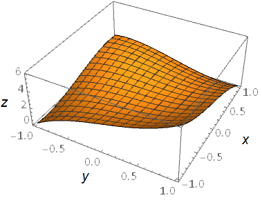
Fig. 1.1 A plot of the function $f(x,\, y) = x^3 - y^3 - 2xy + 2$, along with lines of constant $x,\,y$.¶

Just like the one variable derivative, there is a limit definition for partial derivatives for a function $f = f(x,\,y)$:

\[\begin{split}\frac{\partial f}{\partial x} &= \lim_{\Delta x \rightarrow 0} \left[\frac{f(x + \Delta x,\, y) - f(x,\, y)}{\Delta x} \right]\\ \frac{\partial f}{\partial y} &= \lim_{\Delta x \rightarrow 0} \left[\frac{f(x,\, y + \Delta y) - f(x,\, y)}{\Delta y} \right]\end{split}\]

By way of examples, we can calculate all the first partial derivatives $\partial/\partial x,\, \partial/\partial y$ for the following functions:

$f(x,\,y) = 3x^3 y^2 + 2 y $

\[\begin{split}\frac{\partial f}{\partial x} &= x^2 y^2, \\ \frac{\partial f}{\partial y} &= 6x^3 y+2\end{split}\]

$f(x,\,y) = x^2 \ln(3x+y)$

\[\begin{split}\frac{\partial f}{\partial x} &= 2x\ln(3x+y) + \frac{3x^2}{3x+y}, \\ \frac{\partial f}{\partial y} &= \frac{x^2}{3x+y}\end{split}\]

$z(x,\,y) = \ln(x+y^2\sin(x))$

\[\begin{split}\frac{\partial z}{\partial x} &= \frac{1+y^2\cos(x)}{x+y^2\sin(x)}, \\ \frac{\partial z}{\partial y} &= \frac{2y\sin(x)}{x+y^2\sin(x)}\end{split}\]

1.2. Second Partial Derivatives¶

The second partial derivatives with respect to $x$ and $y$ are denoted as follows:

\[\begin{split}\frac{\partial^2 f}{\partial x^2} &= \frac{\partial}{\partial x}\left(\frac{\partial f}{\partial x}\right), \\ \frac{\partial^2 f}{\partial y^2} &= \frac{\partial}{\partial y}\left(\frac{\partial f}{\partial y}\right)\end{split}\]

The notation can also be extended to mixed second partial derivative, where we take the $x$ and the $y$ partial derivative:

\[\begin{split}\frac{\partial^2 f}{\partial y \,\partial x} &= \frac{\partial}{\partial y}\left(\frac{\partial f}{\partial x}\right), \\ \frac{\partial^2 f}{\partial x\, \partial y} &= \frac{\partial}{\partial x}\left(\frac{\partial f}{\partial y}\right)\end{split}\]

Notice that we work from the inside out, as with function composition and matrix multiplication. For any well behaved, differntiable and continuous function, these two expressions are always equal. The proof of this result (called Schwarz’s theorem) is quite involved and is beyond the scope of this course.

As an example, lets calculate all second partial derivatives of the function $f(x,y)=3x^3y^2+2y$

\[\begin{split}\frac{\partial f}{\partial x} = 9 x^2 y^2, &\quad&\, \frac{\partial f}{\partial y} = 6 x^3 y + 2, \\ \frac{\partial^2 f}{\partial x^2} = 18x y^2, &\quad&\, \frac{\partial^2 f}{\partial y^2} = 6x^3, \\ \frac{\partial^2 f}{\partial y\,\partial x} = 18x^2 y, &\quad&\, \frac{\partial^2 f}{\partial x\,\partial y} = 18x^2 y \end{split}\]

1.3. A Common Mistake¶

Lets look at the function $f(x,\, y) = x^2 y^3 + x + y$ at the point $(1,\, 1)$, calculating the mixed partial derivative:

\[\frac{\partial^2}{\partial y\,\partial x}(x^2 y^3 + x + y)\]

we could argue that we follow the process:

Put $y=1$ into the function and then differentiate with respect to $x$ to obtain:

\[\frac{\partial}{\partial x}(x^2+x+1)=2x\]

Then put $x=1$ into this function and differentiate with respect to $y$ to obtain:

\[\frac{\partial}{\partial y}(2)=0\]

The result is wrong, because we took $y=1$ before differentiating with respect to $y$ - to avoid mistakes of this nature, we should always perform differentiation first and only substitute in the values in the very last step. The correct result is:

\[\Bigg[\frac{\partial^2}{\partial y\,\partial x}\left(x^2 y^3 +x+y\right)\Bigg]_{(1,1)} = \Bigg[\frac{\partial }{\partial y}(2xy^3+1)\Big]_{(1,1)} = \Big[6xy^2\Bigg]_{(1,1)} = 6\]

1.4. Notation for Partial Derivatives¶

Partial derivatives are commonly denoted using subscript notation:

\[\begin{split}f_x=\frac{\partial f}{\partial x}, &\quad&\, f_y=\frac{\partial f}{\partial y}, \\ \quad f_{xx}=\frac{\partial^2 f}{\partial x^2} &\quad&\, f_{yy}=\frac{\partial^2 f}{\partial y^2}\end{split}\]

For mixed derivatives the order or subscripts is from left to right:

\[\begin{split}f_{xy} &= (f_x)_y = \frac{\partial^2 f}{\partial y\, \partial x}, \\ f_{yx} &= (f_y)_x = \frac{\partial^2 f}{\partial x\, \partial y}\end{split}\]

You will likely come across yet more alternative notations in the literature, another common one being:

\[D_x=\frac{\partial}{\partial x}\]

1.5. Multivariable Chain Rule¶

We now consider a function $f(x,\,y)$ subjected to small variations in both $x$ and $y$ as shown in Fig. 1.2.

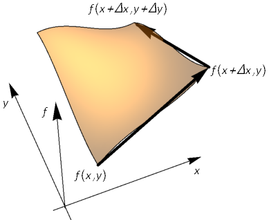
Fig. 1.2 Showing the variations $f(x+\Delta x, \,y+\Delta y)$ in two steps.¶

Loosely speaking, the total change in the function $f(x,\, y)$ is the sum of changes due to each variable:

\[\Delta f = \frac{\partial f}{\partial x}\Delta x + \frac{\partial f}{\partial y}\Delta y\]

If we now suppose that we parameterise $x=x(u,\, v)$ and $y=y(u,\, v)$ then we may similarly write $\Delta x$ and $\Delta y$ as the sum of changes due to variables $u$ and $v$:

\[\Delta f = \frac{\partial f}{\partial x}\left[\frac{\partial x}{\partial u}\Delta u +\frac{\partial x}{\partial v}\Delta v\right] + \frac{\partial f}{\partial y}\left[\frac{\partial y}{\partial u}\Delta u +\frac{\partial y}{\partial v}\Delta v\right]\]

Holding $v$ constant in this expression ($\Delta v=0$) gives:

\[\frac{\Delta f}{\Delta u}=\frac{\partial f}{\partial x}\frac{\partial x}{\partial u}+\frac{\partial f}{\partial y}\frac{\partial y}{\partial u}\]

Holding $u$ constant in this expression ($\Delta u=0$) gives:

\[\frac{\Delta f}{\Delta v}=\frac{\partial f}{\partial x}\frac{\partial x}{\partial v}+\frac{\partial f}{\partial y}\frac{\partial y}{\partial v}\]

This was a somewhat hand-waving argument, but the results are valid in the limit $\Delta u\rightarrow 0, \, \Delta v\rightarrow 0$ and can be proved using the limit definition of the derivative and from this we obtain the multivariable chain rule.

If $f = f(x,\, y)$ where $x=x(u,\, v)$ and $y=y(u,\, v)$ then:

\[\begin{split}\frac{\partial f}{\partial u} &= \frac{\partial f}{\partial x}\frac{\partial x}{\partial u} + \frac{\partial f}{\partial y}\frac{\partial y}{\partial u}\\ \frac{\partial f}{\partial v} &= \frac{\partial f}{\partial x}\frac{\partial x}{\partial v} + \frac{\partial f}{\partial y}\frac{\partial y}{\partial v}\end{split}\]

Many student’s first go at encountering this rule often think that it “can’t be right”, because replacing the partial derivatives with differences gives:

\[\Delta f = \frac{\Delta f}{\Delta x}\Delta x + \frac{\Delta f}{\Delta y}\Delta y\]

which suggests the result $\Delta f = 2\Delta f$. However, this misunderstanding comes from ambiguity in writing $\Delta f$.

On the left-hand side it means changes in $f$ dues to variations in both $x$ and $y$, whilst in $f_x$ and $f_y$ the changes are due to only one of these variables, whilst the other is held constant. Written formally:

\[\begin{split}\frac{\partial f}{\partial u} &= \lim_{\Delta u\rightarrow 0}\frac{f(x(u+\Delta u,v),y(u+\Delta u,v))-f(x(u,v),y(u,v))}{\Delta u}, \\ \frac{\partial f}{\partial x} &= \lim_{\Delta x\rightarrow 0}\frac{f(x+\Delta x,y)-f(x,v)}{\Delta x} =\lim_{\Delta u\rightarrow 0}\frac{f(x(u+\Delta u,v),y(u,v))-f(x(u,v),y(u,v))}{\Delta u}\end{split}\]

The lesson here is - it is dangerous to treat partial derivatives as fractions!

1.6. Dependency Trees¶

The multivariate chain rule can be illustrated as a dependency tree, in Fig. 1.3, where we examine $f(x,\, y)$ with $x = x(u,\, v)$ and $y = y(u,\, v)$:

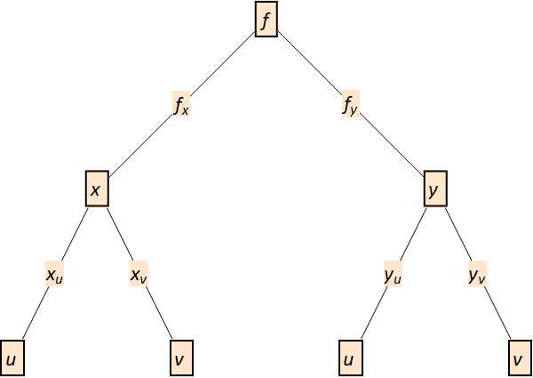
Fig. 1.3 Dependency tree for first derivatives.¶

For instance, if we follow the dependency routes involving $u$, we get $f_u = f_x\, x_u + f_y\, y_u$.

We can do the same thing for the second derivatives (a repeat application of the chain rule), in Fig. 1.4.

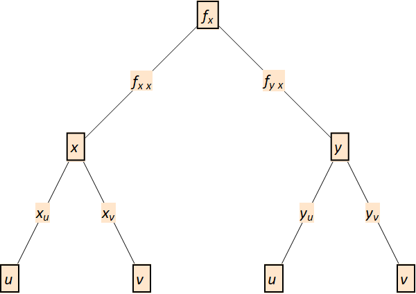
Fig. 1.4 Dependency tree for second derivatives.¶

As an example lets look at the function $f(x,y)=x^2 y+y^2$, if we have $x = u+v$ and $y = u-v$, then we can calculate $f_u,\, f_v$ using dependency trees:

\[\begin{split}f_u = f_x\, x_u + f_y\, y_u\\ f_v = f_x\, x_v + f_y\, y_v\end{split}\]

meaning that:

\[\begin{split}f_x &= 2xy, \\ f_y &= x^2+2y \\ x_u=1, &\quad&\, x_v=1, \\ y_u=1, &\quad&\, y_v=-1\end{split}\]

Putting these results together:

\[\begin{split}f_u = f_x\, x_u + f_y\, y_u &= 2xy+(x^2+2y) = 2(u+v)(u-v)+(u+v)^2+2(u-v)\\ f_v = f_x\, x_v + f_y\, y_v &= 2xy-(x^2+2y) = 2(u+v)(u-v)-(u+v)^2-2(u-v)\end{split}\]

We can also use techniques to simplify calculating more complicated derivatives, for example for the function:

\[f(x,\, y) = \sin\left(x^2+2xy\right)+(x-y)^2\]

To find $f_x$, we can let $u = x^2 + 2xy$, $v = x-y$, then:

\[f_x = f_u\, u_x +f_v\, v_x = \cos(u)(2x+2y)+2v = 2(x+y)\cos(x^2+2xy) + 2(x-y)\]

1.7. Exact derivatives and differentials¶

The multivariate chain rule is sometimes written in differential form:

\[\mathrm{d}F=\frac{\partial F}{\partial x}\,\mathrm{d}x+\frac{\partial F}{\partial y}\,\mathrm{d}y\]

Comparing this result to a general expression of the form:

\[\mathrm{d}F=A(x,y)\,\mathrm{d}x+B(x,y)\,\mathrm{d}y\]

which tells us that:

\[A = \frac{\partial F}{\partial x}, \quad B=\frac{\partial F}{\partial y}\]

For these two results to be consistent, we require that the mixed second derivatives of $F$ are equal, in accordance with Schwarz’ theorem. Therefore, we require that:

\[\frac{\partial A}{\partial y}\equiv\frac{\partial B}{\partial x}\]

If the differential is exact, then it can be exactly integrated to obtain a solution $F$. Whilst you might not be asked to obtain solutions for $F$, you may be asked to verify if a differential expression is exact by testing this condition.

As an example, lets try showing that:

\[(y\cos{x}+\sin{y}+y)\,\mathrm{d}x + (\sin{x}+x\cos{y}+x)\,\mathrm{d}y\]

is an exact differential.

The expression is of the form:

\[A(x,\, y)\,\mathrm{d}x + B(x,\, y)\,\mathrm{d}y = 0\]

where we have taken:

\[\begin{split}A &= y\cos{x}+\sin{y}+y \\ B &= \sin{x}+x\cos{y}+x\end{split}\]

Then if we examine the conditions:

\[\begin{split}\frac{\partial A}{\partial y} &= \cos{x} + \cos{y} + 1\\ \frac{\partial B}{\partial x} &= \cos{x} + \cos{y} + 1\\ \Rightarrow \frac{\partial A}{\partial y} &= \frac{\partial B}{\partial x}\end{split}\]

and therefore the expression is exact.

1.7.1. Solving 1st order ODEs *¶

Optionally, this result could be used to solve the nonlinear 1st order ODE:

\[\frac{\mathrm{d}y}{\mathrm{d}x} + \frac{y\cos{x} + \sin{y} + y}{\sin{x} + x\cos{y} + x}=0\]

We can rewrite this in the form:

\[\begin{split}(y\cos{x} + \sin{y} + y)\,\mathrm{d}x + (\sin{x} + x\cos{y} + x)\,\mathrm{d}y = 0\\\end{split}\]

and if we let:

\[\begin{split}A &= y\cos{x} + \sin{y} + y = \frac{\partial F}{\partial x}, \\ B &= \sin{x} + x\cos{y} + x = \frac{\partial F}{\partial y}\end{split}\]

where $F(x,\,y)$ is to be determined.

By integrating $A$ w.r.t. $x$ and $B$ w.r.t $y$ we obtain:

\[\begin{split}F &= y\sin{x} + x\sin{y} + xy + F_1(y)\\ F &= y\sin{x} + x\sin{y} + xy + F_2(x)\end{split}\]

where we introduced the arbitrary functions $F_1,\, F_2$. For consistency we require that $F_1(y) = F_2(x) = \mathrm{const.}$, this allows us to write the given ODE as:

\[\frac{\mathrm{d}}{\mathrm{d}x}\left(y\sin{x}+x\sin{y}+xy\right)=0\]

and so the solution is given by:

\[y\sin{x}+x\sin{y}+xy=\mathrm{const.}\]

That is, $F(x,\, y) = 0$ where:

\[F(x,\, y) = y\sin{x} + x\sin{y} + xy + k\]

and $k$ here is an arbitrary constant.

1.8. Stationary Points¶

If we think about stationary points in multivariable calculus:

When $\frac{\partial f}{\partial x}=0$ the function is stationary (flat) with respect to the $x$-axis
When $\frac{\partial f}{\partial y}=0$ the function is stationary (flat) with respect to the $y$-axis

Recall from the multivariate chain rule:

\[\mathrm{d}f = \frac{\partial f}{\partial x}\mathrm{d}x+\frac{\partial f}{\partial y}\mathrm{d}y\]

then it is apparent that when both $\frac{\partial f}{\partial x}=0$ AND $\frac{\partial f}{\partial y}=0$, then the instantaneous rate of change of $f$ is zero in any direction.

As an example, lets think again about the function in Fig. 1.1, $f(x,\, y) = x^3 - y^3 - 2xy + 2$ can be found by solving $f_x = f_y = 0$ simultaneously:

\[\begin{split}3y^2+2x&= 0\\ 3x^2-2y&= 0\end{split}\]

In general, it may be very difficult (or impossible!) to solve nonlinear equations by hand, and so we would need to resort to numerical methods. In this case, however, we can proceed by rearranging one of the equations to substitute into the other, to obtain

\[3\left(\frac{3}{2}x^2\right)^2+2x=0 \quad \leftrightarrow\quad x(27x^3+8)=0\]

This equation has solutions $x=0$ and $x=-\frac{2}{3}$, as well as a complex conjugate pair of solutions $\frac{1}{3}(1\pm\sqrt{3}i)$, which we will discard here.

Hence, the stationary points are $(0,\, 0,\, 2)$ and $\left(-\frac{2}{3},\, \frac{2}{3},\, \frac{62}{27}\right)$, where we write $(x,\, y,\, f)$

1.8.1. Classification of Stationary Points¶

For a function $f(x,\,y)$, we might expect to classify stationary points using $f_{xx}$ and $f_{yy}$. After all:

$f_{xx}$ tells us the function concavity parallel to the $y$ axis
$f_{yy}$ tells us the function concavity parallel to the $x$ axis
If the function is concave up in both the $x$ and $y$ directions through a stationary point, then intuition tells us that this is a local minimum.
If the function is concave down in both the $x$ and $y$ directions through a stationary point, then our intuition tells us that this is a local maximum.

We can examine this through some example functions,

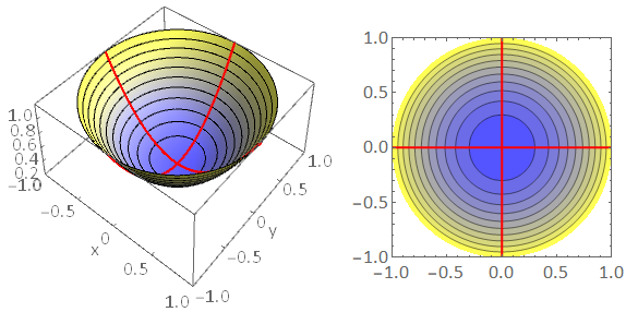
Fig. 1.5 Left: Local minimum of a function $f(x,y)$. The red lines illustrate the concave upwards behaviour in the $x$ and $y$ directions $f_{xx}>0$, $f_{yy}>0$. The black contours are plotted on the surface at constant height. Notice that they form rings around the stationary point. Right: Contour plot showing locations in the $(x,y)$ plane where $f(x,y)$ is constant. The colour scheme blue$\rightarrow$yellow is used to indicate the height of the contours, with yellow representing points at higher elevation. The contour plot shows that the function is increasing in all directions away from the stationary point.¶

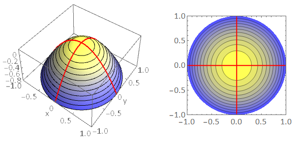
Fig. 1.6 Left Panel: Local maximum of a function $f(x,y)$. The red lines illustrate the concave downwards behaviour in the $x$ and $y$ directions $f_{xx}<0$, $f_{yy}<0$. The black contours are plotted on the surface at constant height. Notice that they form rings around the stationary point. Right Panel: Contour plot showing locations in the $(x,y)$ plane where $f(x,y)$ is constant. The colour scheme blue$\rightarrow$yellow is used to indicate the height of the contours, with yellow representing points at higher elevation. The contour plot shows that the function is decreasing in all directions away from the stationary point.¶

However, a local maximum/minimum is not the only type of stationary point that a surface $f(x,\,y)$ can have. For instance, a surface may have a stationary point that sits where the function is concave upwards with respect to one axis and concave downwards with respect to the other axis. This type of point is called a saddle point (it looks like a saddle for a horse). The figure below shows an example:

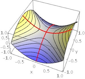
Fig. 1.7 Left Panel: Saddle point of a function $f(x,\,y)$. The red lines illustrate the concave upwards/downwards behaviour in the $x$ and $y$ directions $f_{xx}>0$, $f_{yy}<0$. The black contours are plotted on the surface at constant height. Notice that the contours cross at a saddle point. Right Panel: Contour plot showing locations in the $(x,\,y)$ plane where $f(x,\,y)$ is constant. The colour scheme blue$\rightarrow$yellow is used to indicate the height of the contours, with yellow representing points at higher elevation. The contour plot also shows the function concavity in the $x,\, y$ directions.¶

We conclude that at a stationary point, if $f_{xx}$ and $f_{yy}$ are opposite sign, then the point is a saddle point. However, the converse is not necessarily true! It turns out that we can have a saddle point where $f_{xx}$ and $f_{yy}$ are both the same sign (or even when they are both zero). An example is illustrated in the figure below. In this case the saddle point is not aligned squarely with the $(x,\,y)$ coordinate directions.

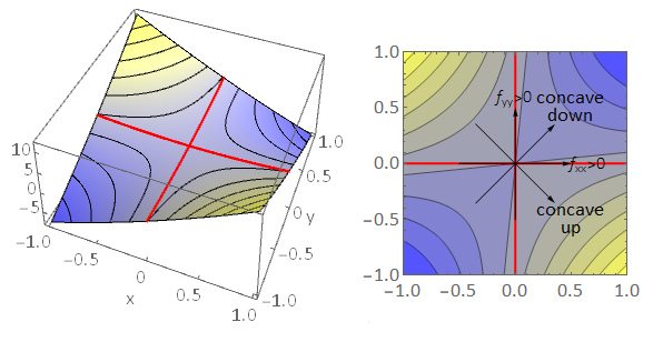
Fig. 1.8 Left Panel: Saddle point of a function $f(x,y)$ that is not aligned squarely with the $x,\,y$ axes. The red lines illustrate the concave upwards behaviour in the $x$ and $y$ directions $f_{xx}>0$, $f_{yy}>0$. The curve has concave down behaviour at approximately $45^{\circ}$ to the $x$-axis. Right Panel: Contour plot showing locations in the $(x,\,y)$ plane where $f(x,\,y)$ is constant. The colour scheme blue$\rightarrow$yellow is used to indicate the height of the contours, with yellow representing points at higher elevation. The competing concave up/down behaviour is apparent from the contour plot.¶

So, it turns outs that the condition for a maximum/minimum is more complicated than we first thought! A valid classification algorithm is presented in the box below.

The result can be proved by utilising a multivariate Taylor series expansion about the stationary point and retaining terms only up to quadratic order so that the shape of the function may be inferred from the properties of a quadratic. Neglecting the higher order terms in the expansion is justified in the limit approaching the stationary point. We have not studied the multivariate chain rule, so the proof is not presented here.

1.8.2. Hessian Matrix¶

At a stationary point, $f_x(x_0,y_0)=f_y(x_0,y_0)$, we calculate the determinant of the Hessian matrix at $H(x_0,\,y_0)$:

\[\begin{split}\det(H) = \begin{vmatrix} f_{xx}&f_{xy}\\ f_{yx}&f_{yy} \end{vmatrix}=f_{xx}f_{yy}-(f_{xy})^2\end{split}\]

This can have a few different outcomes:

If $\det(H(x_0,\,y_0))>0$ then the point is a local max/min, depending on the signs of $f_{xx}$ and $f_{yy}$.
If $\det(H(x_0,\,y_0))<0$ then the point is a saddle.
If $\det(H(x_0,\,y_0))=0$ then the test is inconclusive and further analysis is needed.

Lets classify the stationary points of the function $f=x^3-y^3-2xy+2$, we already found that the stationary points are located at $(0,0,2)$ and $\left(-\frac{2}{3},\frac{2}{3},\frac{62}{27}\right)$.

Calculating the Hessian determinant components $f_{xx}=6x, \quad f_{yy}=-6y, \quad f_{xy}=f_{yx}=-2$ and therefore:

\[\begin{split}\det(H(x,y)) = \begin{vmatrix} 6x &-2 \\ -2 &-6y \end{vmatrix}=-36xy-4\end{split}\]

$\det(H(0,0))=-4<0$ so the origin is a saddle point.

$\det\biggr(H\biggr(-\frac{2}{3},\frac{2}{3}\biggr)\biggr)=12>0$ and $f_{xx}\left(-\frac{2}{3},\frac{2}{3}\right)<0$, so the point $\left(-\frac{2}{3}\frac{2}{3}\right)$ is a local maximum.

A contour plot of the function, shown in Fig. 1.9, confirms these findings.

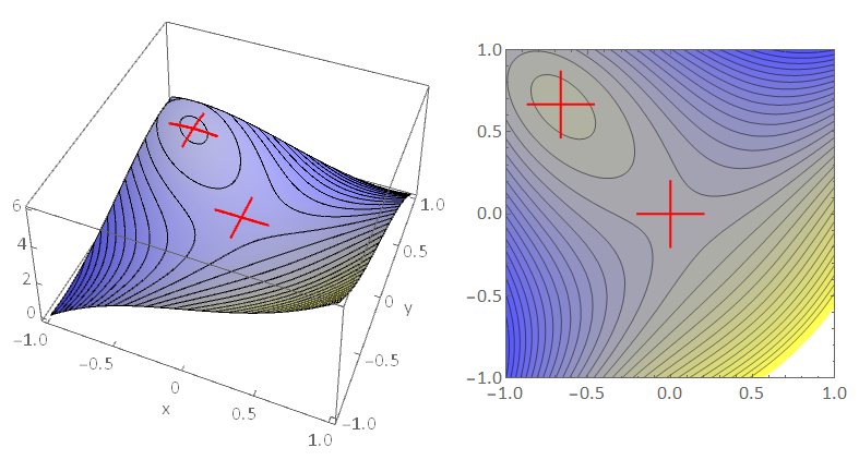
Fig. 1.9 Contour plot of $f=x^3-y^3-2xy+2$, showing stationary points clearly.¶

Mathematics for Natural Sciences 2

Multivariable Calculus

Contents