.md .pdf

Contents

3. Vectors and Vector Algebra

We can think of vectors at their heart as directions being given to get between two points in space. If we have to move in one, two or three dimensions, along spatially flat or curved surfaces, we can attempt to give directions. At the heart of a any vector system are the basis vectors, these give us the funadmental possible directions within a vector space, which any vector can be decompsoed into a weighted sum of.

In the Cartesian coordinate system, in three dimensions the basis vectors are given as:

\[\begin{split}\hat{\bf x} = \,\begin{pmatrix} 1 \\ 0 \\ 0 \end{pmatrix}, \quad \hat{\bf y} = \,\begin{pmatrix} 0 \\ 1 \\ 0 \end{pmatrix}, \quad \hat{\bf z} \,\begin{pmatrix} 0 \\ 0 \\ 1 \end{pmatrix}\end{split}\]

and when we switch to different coordinate systems, we will consider how these change. Note that a variety of different letters are employed for the Cartessian system:

\[\begin{split}\hat{\bf x} &= {\bf e_x} = \vec{x} = \hat{\bf i}\\ \hat{\bf y} &= {\bf e_y} = \vec{y} = \hat{\bf j}\\ \hat{\bf z} &= {\bf e_z} = \vec{z} = \hat{\bf k}\end{split}\]

To see how these visually fit together, see Fig. 3.1. We note that all the coordinates meet at right angles and that we have defined right handed axes.

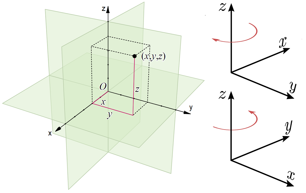
Fig. 3.1 Left Pane: Graphical breakdown of the Cartesian coordinate system with vector path in red, Right Pane: The differences between left handed (top) and right handed (bottom) axes.

We can also write coordinates in so-called index notation:

\[x_i = \left(\hat{\bf x},\, \hat{\bf y},\, \hat{\bf z}\right)\]

where the value of \(i = \in \{1,\,2,\,3\}\) denotes the specific basis vector.

3.1. Addition and Scaling of Vectors

If we start with the basis vectors as building blocks of our coordinate system, then we can write any three dimensional Cartesian coordinate in terms of weighted basis vectors, we can see this in Fig. 3.2.

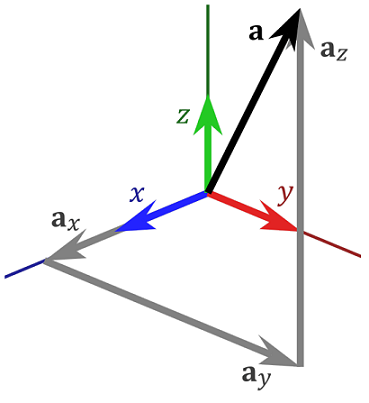
Fig. 3.2 Breakdown of vector \(\bf a = a_x \,\hat{\bf x} + a_y \,\hat{\bf y} + a_z \,\hat{\bf z}\).

As an example we can define two vectors \(\bf v_1,\, v_2\)

\[\begin{split}{\bf v}_1 &= \begin{pmatrix} 3 \\ 4 \\ 12 \end{pmatrix} = 3\hat{\bf x} + 4\hat{\bf y} + 12\hat{\bf z}\\ {\bf v}_2 &= \begin{pmatrix} 5 \\ 12 \\ 13 \end{pmatrix} = 5\hat{\bf x} + 12\hat{\bf y} + 13\hat{\bf z}\end{split}\]

Then we can add or sutract these vectors:

\[\begin{split}{\bf v}_1 + {\bf v}_2 &= \begin{pmatrix} 3 \\ 4 \\ 12 \end{pmatrix} + \begin{pmatrix} 5 \\ 12 \\ 13 \end{pmatrix} = \begin{pmatrix} 8 \\ 16 \\ 25 \end{pmatrix} = 8\hat{\bf x} + 16\hat{\bf y} + 25\hat{\bf z}\\ {\bf v}_2 - {\bf v}_1 &= \begin{pmatrix} 5 \\ 12 \\ 13 \end{pmatrix} - \begin{pmatrix} 3 \\ 4 \\ 12 \end{pmatrix} = \begin{pmatrix} 2 \\ 8 \\ 1 \end{pmatrix} = 2\hat{\bf x} + 8\hat{\bf y} + \hat{\bf z} \end{split}\]

Likewise we can scale each of the vectors and then proceed to add them:

\[\begin{split}2{\bf v}_1 + 3{\bf v}_2 &= 2\begin{pmatrix} 3 \\ 4 \\ 12 \end{pmatrix} + 3\begin{pmatrix} 5 \\ 12 \\ 13 \end{pmatrix} = \begin{pmatrix} 21 \\ 44 \\ 63 \end{pmatrix} = 21\hat{\bf x} + 44\hat{\bf y} + 49\hat{\bf z}\end{split}\]

3.2. Magnitude of a Vector

Given some vector, which will take us some distance from two points in space, we can find the shortest path length between the points.

In two dimensions this would just follow Pythagoras’s theorem:

\[{\bf v} = a_x\hat{\bf x} + a_y\hat{\bf y} v_3 = |{\bf v}| = \sqrt{{a_x}^2 + {a_y}^2}\]

and in three dimensions a similar relation holds (which we can prove geometrically:

\[{\bf v} = a_x\hat{\bf x} + a_y\hat{\bf y} + a_z\hat{\bf z} v_3 = |{\bf v}| = \sqrt{{a_x}^2 + {a_y}^2 + {a_z}^2} \]

As an example lets consider \(\bf v_1\):

\[|3\hat{\bf x} + 4\hat{\bf y} + 12\hat{\bf z}| = \sqrt{3^2 + 4^2 + 12^2} = 13\]

3.3. Normalised Vectors

Each of the basis vectors is a normalised vector \(|\hat{\bf x}| = |\hat{\bf y}| = |\hat{\bf z}| = 1\), however if we have a more general vector \({\bf v} = a_x\hat{\bf x} + a_y\hat{\bf y} + a_z\hat{\bf z}\) moving in some direction, we can also construct a normalised vector:

\[\hat{\bf v} = \frac{\bf v}{|\bf v|} = \frac{a_x\hat{\bf x} + a_y\hat{\bf y} + a_z\hat{\bf z}}{\sqrt{{a_x}^2 + {a_y}^2 + {a_z}^2}}\]

As an example lets consider \(\bf v_1\):

\[\hat{\bf v_1} = \frac{\bf v_1}{|\bf v_1|} = \frac{3\hat{\bf x} + 4\hat{\bf y} + 12\hat{\bf z}}{\sqrt{3^2 + 4^2 + 12^2}} = \frac{1}{13}\left(3\hat{\bf x} + 4\hat{\bf y} + 12\hat{\bf z}\right)\]

3.4. Scalar Product / Dot Product

3.4.1. Geometric Definiton

Lets consider two vectors \(\bf A,\, B\), as shown in Fig. 3.3. We can consider the scalar projection of the vector \(\bf B\) on to the vector \(\bf A\), where we resolve the parallel components of \(\bf B\) in the direction of vector \(\bf A\).

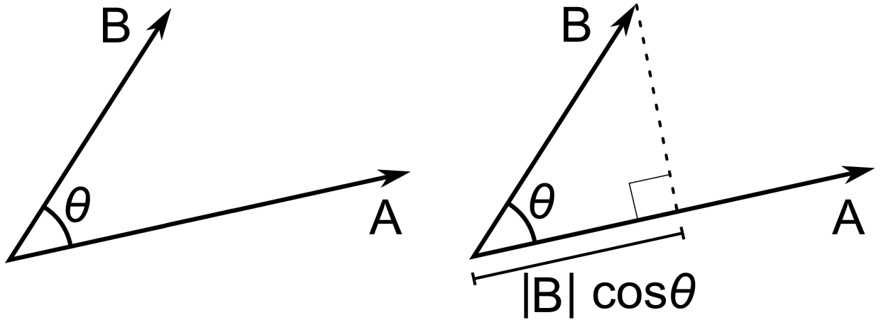
Fig. 3.3 Left Pane: Vectors \(\bf A,\, B\) which share a common coordinate and span an angle \(\theta\) between them, Right Pane The scalar projection of the vector \(\bf B\) on to the vector \(\bf A\), which by trigonometry gives the length \(|{\bf B}| \cos\theta\).

If we multiply these two distances, this is Scalar Product of the vectors:

\[{\bf A \cdot B} = |{\bf A}||{\bf B}|\cos(\theta)\]

also known as the Dot Product.

So we can calculate the scalar projection of \(\bf B\) onto vector \(\bf A\) using \({\bf A \cdot B} / |{\bf A}|\). Likewise we can think about the scalar projection of \(\bf A\) onto the vector \(\bf B\), using \({\bf A \cdot B} / |{\bf B}|\).

We can also find the magntiude of a vector from \(\bf A \cdot A = |A|^2 \).

3.4.2. Algebraic Definition

There is another perspective on the scalar product, which is for two vectors with components:

\[\begin{split}{\bf A} &= a_x\,\hat{\bf x} + a_y\,\hat{\bf y} + a_z\,\hat{\bf z} = \begin{pmatrix} a_x \\ a_y \\ a_z \end{pmatrix} \\ {\bf B} &= b_x\,\hat{\bf x} + b_y\,\hat{\bf y} + b_z\,\hat{\bf z} = \begin{pmatrix} b_x \\ b_y \\ b_z \end{pmatrix}\end{split}\]

then the dot product can be found by:

\[{\bf A \cdot B} = a_x\,b_x + a_y\,b_y + a_z\,b_z= \sum_{i=1}^3 a_i\,b_i\]

where the last expression uses the index notation.

3.4.3. Properties of the Dot Product

The dot product of two vectors \(\bf a,\, b\) have the following mathematical properties:

• Commutative: \(\mathbf {a} \cdot \mathbf {b} = \mathbf {b} \cdot \mathbf {a}\)

• Distributive over Vector Addition: \( \mathbf {a} \cdot (\mathbf {b} +\mathbf {c} )=\mathbf {a} \cdot \mathbf {b} +\mathbf {a} \cdot \mathbf {c}\)

• Bilinear: \( \mathbf {a} \cdot (r\mathbf {b} +\mathbf {c} )=r(\mathbf {a} \cdot \mathbf {b} )+(\mathbf {a} \cdot \mathbf {c} )\)

• Scalar Multiplication: \( (c_{1}\mathbf {a} )\cdot (c_{2}\mathbf {b} )=c_{1}c_{2}(\mathbf {a} \cdot \mathbf {b} )\)

• Orthogonal: Two non-zero vectors \(\bf a,\, b\) are orthogonal if and only if \(\bf a \cdot b = 0\).

3.5. Vector Product / Cross Product

3.5.1. Geometric Definition

Unsurprisingly we can also make a vector product that results in a vector, rather than a scalar. This Vector Product, also known as the Cross Product, can be constructed from the basis vectors:

\[\begin{split}\hat{\bf x} \times \hat{\bf y} &= \hat{\bf z} \\ \hat{\bf y} \times \hat{\bf z} &= \hat{\bf x} \\ \hat{\bf z} \times \hat{\bf x} &= \hat{\bf y} \end{split}\]

In general however we write the cross product between two vectors as a new vector, normal to the other two (following the right hand rule), as depicted in Fig. 3.4.

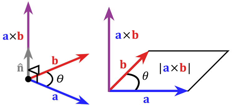
Fig. 3.4 Left Pane: Graphical depiction of the cross product, producing a vector \(\bf a \times b\) which is normal to both \(\bf a,\, b\), Right Pane: The area of the parallogram produced by vectors \(\bf a,\, b\) is found from \(|\bf a \times b|\)

This means that if vectors span an angle \(\theta\), then we need to resolve the perpendicular component:

\[{\bf a \times b} = {\bf |a||b|}\sin(\theta)\,\hat{\bf n}\]

where \(\hat{\bf n}\) is vector which is normal to both \(\bf a,\, b\).

Because the cross product follows the right hand rule for axes, it is anti-commutative:

\[\bf a \times b = -\,b \times a\]

We also find the at the cross product is distributive over addition,

\[\mathbf {a} \times (\mathbf {b} +\mathbf {c} )=(\mathbf {a} \times \mathbf {b} )+(\mathbf {a} \times \mathbf {c} )\]

and compatible with scalar multiplication:

\[(r\,\mathbf {a} )\times \mathbf {b} =\mathbf {a} \times (r\,\mathbf {b} )=r\,(\mathbf {a} \times \mathbf {b} )\]

Likewise since the vector magnitude depends on the angle between the two vectors, if we cross a vector with itself (or another vector that is parallel / anti-parallel), the answer is zero:

\[\bf a \times a = 0\]

where \(\bf 0\) is a zero vector.

3.5.2. Algebraic Definition

Once again there is also an algebraic route to the cross product, this is based on the vector components.

Since the cross product is distributive over addition we find that:

\[\begin{split} \mathbf{a}\times\mathbf{b} = {} &(a_x\,\hat{\bf x} + a_y\,\hat{\bf y} + a_z\,\hat{\bf z}) \times (b_x\,\hat{\bf x} + b_y\,\hat{\bf y} + b_z\,\hat{\bf z})\\ = {} &a_x\,b_x(\hat{\bf x} \times \hat{\bf x}) + a_x\,b_y(\hat{\bf x} \times \hat{\bf y}) + a_x\,b_z(\hat{\bf x} \times \hat{\bf z}) + {}\\ &a_y\,b_x(\hat{\bf y} \times \hat{\bf x}) + a_y\,b_y(\hat{\bf y} \times \hat{\bf y}) + a_y\,b_z(\hat{\bf y} \times \hat{\bf z}) + {}\\ &a_z\,b_x(\hat{\bf z} \times \hat{\bf x}) + a_z\,b_y(\hat{\bf z} \times \hat{\bf y}) + a_z\,b_z(\hat{\bf z} \times \hat{\bf z})\\\end{split}\]

If we follow through our rules for computing the cross products of basis vectors, we find this simplifies to:

\[\begin{split} \mathbf{a}\times\mathbf{b} = {} &a_x\,b_x(0) + a_x\,b_y(\hat{\bf z}) + a_x\,b_z(-\hat{\bf y}) + {}\\ &a_y\,b_x(-\hat{\bf z}) + a_y\,b_y(0) + a_y\,b_z(\hat{\bf x}) + {}\\ &a_z\,b_x(\hat{\bf y}) + a_z\,b_y(-\hat{\bf x}) + a_z\,b_z(0)\\ = {} &(a_y\,b_z - a_z\,b_y)\hat{\bf x} + (a_z\,b_x - a_x\,b_z)\hat{\bf y} + (a_x\,b_y - a_y\,b_x)\hat{\bf z} \end{split}\]

Finding the cross product can also be found using a matrix determinant:

\[\begin{split} \mathbf{a}\times\mathbf{b} = \begin{vmatrix} \hat{\bf x} & \hat{\bf y} & \hat{\bf z} \\ a_x & a_y & a_z \\ b_x & b_y & b_z \end{vmatrix}\end{split}\]

which by the cofactor method along the first row produces:

\[\begin{split} \mathbf{a}\times\mathbf{b} &= \begin{vmatrix} a_y & a_z \\ b_y & b_z \end{vmatrix}\hat{\bf x} - \begin{vmatrix} a_x & a_z \\ b_x & b_z \end{vmatrix}\hat{\bf y} + \begin{vmatrix} a_x & a_y b_x & b_y \end{vmatrix}\hat{\bf z} \\ &= (a_y\,b_z - a_z\,b_y)\hat{\bf x} - (a_x\,b_z - a_x\,b_z)\hat{\bf y} + (a_x\,b_y - a_y\,b_x)\hat{\bf z} \end{split}\]

which we find are equivalent definitions.

3.6. Triple Vector Products

Now that we have multiplcation of two vectors formalised, we find that multiplying three vectors also leads to some further geometric and algebraic ideas.

3.6.1. Triple Scalar Product

Here we have three vectors \(\bf a, \,b,\,c\) composed so that

\[\bf a \cdot (b \times c)\]

since the combination of \(\bf b \times c\) produces a vector, which we can then do a scalar multiplcation with \(\bf a\). Therefore this produces a scalar result.

Geometrically this is related to the parallepiped, as depicted in Fig. 3.5, where the magnitude of this result is the shapes volume:

\[V = |{\bf a \cdot (b \times c)}|\]

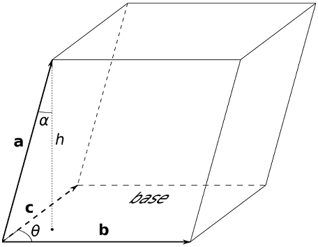
Fig. 3.5 A parallepiped, composed from three vectors \(\bf a, \,b,\,c\).

We can also evaluate the triple scalar product from a matrix determinant:

\[\begin{split} {\bf a \cdot (b \times c)} = \mathbf{a}\times\mathbf{b} = \begin{vmatrix} a_x & a_y & a_z \\ b_x & b_y & b_z \\ c_x & c_y & c_z \\ \end{vmatrix}\end{split}\]

3.6.2. Triple Vector Product

Unsurprisingly we can also find an expression for the vector product between three vectors \(\bf a, \,b,\,c\):

\[\bf a \times (b \times c) = (a\cdot c)b - (a \cdot b)c\]

which is useful particularly when we want to work out results like:

\[\bf \nabla \times \nabla \times A = \nabla(\nabla \cdot A) - (\nabla\cdot \nabla)A = \nabla(\nabla \cdot A) - \nabla^2 A\]

which will be useful later!

3.7. Vector Lines and Planes

We can identify points in space using their position vectors, which are typically denoted by

\[\begin{split}{\bf r} =\left(\begin{array}{c}x\\y\\z\end{array}\right)\end{split}\]

This gives us two ways of writing down the equations of lines and planes:

• Vector Form: in terms of the position vector \(\bf r\),

• Scalar Form: in terms of the coordinates \(x,\, y,\, z\).

In what follows, we will write the equations using both conventions. You will see that sometimes it is easier to work with the scalar equations and other times it is easier to work with the vector equations.

3.7.1. Equation of a Line

The vector equation of a line can be obtained from a known point on the line and a known vector parallel to the line. Equivalently, two known points on the line can also be used to find a parallel vector.

We obtain the position vector of the other points by a two step process:

• first carrying from the origin to the known point

• secondly carrying along the line in either direction

This principle is illustrated in Fig. 3.6

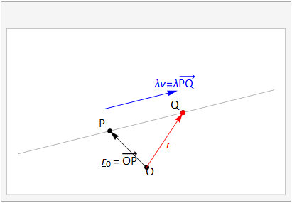
Fig. 3.6 The vector equation of a line passing through two points \(P,\,Q\). The position vector \(\bf r\), shown in red, describes an arbitrary point on the line, it can be formed by the sum \({\bf r}={\bf r}_0+\lambda{\bf v}\).

An arbitrary scalar parameter \(\lambda\) controls how far along the line we move, and if it is negative then the direction is reversed. The animation shows how the line is described as the parameter \(\lambda\) is varied.

We can also use the vector equation to calculate the corresponding scalar equation. From the vector equation we obtain:

\[\begin{split}\begin{pmatrix} x \\y \\z \end{pmatrix} = \begin{pmatrix} x_0 \\y_0 \\z_0 \end{pmatrix} + \lambda \begin{pmatrix} v_x \\v_y \\v_z \end{pmatrix}\end{split}\]

Equating components on the left and right and rearranging in each equation for \(\lambda\) then gives the result in vector form :

\[{\bf r}={\bf r}_0+\lambda{\bf v}\]

or in scalar form:

\[\frac{x-x_0}{v_x}=\frac{y-y_0}{v_y}=\frac{z-z_0}{v_z}\]

where \({\bf r_0}=\begin{pmatrix} x_0\\y_0\\z_0\end{pmatrix}\) is the position vector of a point on the line, and \({\bf v}=\begin{pmatrix} v_x\\v_y\\v_z\end{pmatrix}\) is a vector parallel to the line. Notice that the special case where \(z\) is constant gives an equation of the form \(y = m x+c\)

As an example, we can wfind the vector equation of the lines \(\frac{3x+1}{2} = \frac{y−1}{2} = \frac{5−z}{3}\), by setting each of these to equal some constant \(\lambda\), hence:

\[\begin{split}x &= \frac{1}{3}(2\lambda-1) = -\frac{1}{3} + \frac{2}{3}\lambda \\ y &= 1 + 2\lambda \\ z &= -(3\lambda -5) = 5 - 3 \lambda\end{split}\]

and therefore the vector equation is:

\[\begin{split}{\bf r} = \begin{pmatrix} -1/3\\1\\5\end{pmatrix} + \lambda \begin{pmatrix} 2/30\\2\\-3\end{pmatrix}\end{split}\]

3.7.2. Equation of a Plane

The vector equation requires either three points (which cannot lie all on the same line), or a point and two non-parallel directions. The vector form of the equation is illustrated in Fig. 3.7.

In this description we carry from the origin to the known point identified by \({\bf r}_0\) and then carry along the resultant of vectors \(\lambda{\bf v}\) and \(\mu{\bf w}\), which span a parallelogram within the plane.

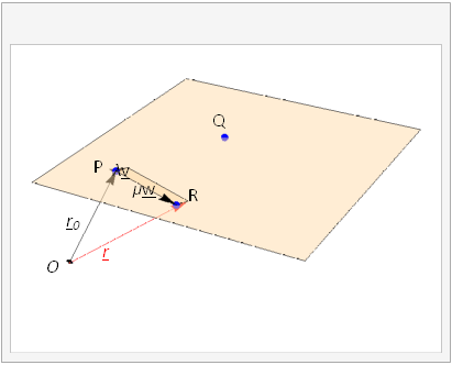
Fig. 3.7 The position vector \({\bf r}\), shown in red, describes an arbitrary point on the plane. It can be formed by the sum \({\bf r}={\bf r}_0+\lambda{\bf v}+\mu{\bf w}\), where \({\bf r}_0=\overrightarrow{OP}\) is a the position vector of one of the known points on the line,\({\bf v}=\overrightarrow{PQ}\) and \({\bf w}=\overrightarrow{PR}\) are known vectors that points in a different directions parallel to the plane. The arbitrary scalar parameters \(\lambda\) and \(\mu\) control how far along the line we carry. The animation shows how the plane is described as the parameters are varied.

Written out in scalar form, the vector equation of a plane gives :

\[\begin{split}\lambda v_x +\mu w_x &= x-x_0\\ \lambda v_y +\mu w_y &= y-y_0\\ \lambda v_z +\mu w_z &= z-z_0\end{split}\]

In principle, we could find the scalar equation for a plane by eliminating the parameters \(\lambda,\mu\) between these equations, which would lead to a relationship of the form \(ax +by+cz=k\). However, we can avoid the messy algebra by obtaining the scalar equation in a different way.

We can find the scalar equation of a plane if we know the position vector \(\bf r_0\) of a point on the surface, and a vector \(n\) that is normal to the surface. Then, \({\bf r}-{\bf r}_0\) lies inside the plane, so it is perpendicular to \(n\).

This gives the result that the scalar equation of a plane is given by:

\[({\bf r}-{\bf r}_0)\cdot{\bf n}=0\]

where \({\bf r}_0\) is the position vector of a point in the plane, and \({\bf n}\) is a vector perpendicular to the plane. We see this depicted in Fig. 3.8.

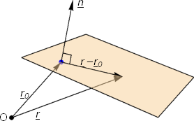
Fig. 3.8 We can find the scalar equation of a plane by using a normal vector \({\bf n}\) and a position vector \({\bf r}_0\). We have \(({\bf r}-{\bf r}_0)\cdot{\bf n}=0\).

Expanding out the scalar product gives:

\[n_x x +n_y y + n_z z = k\]

where \(k=n_x x_0 +n_y y_0 + n_z z+0\)

In the case where we are given two vectors \(v,\,w\) lying inside the plane we can, of course, find a normal vector by making use of the vector product!

So, we could write:

\[({\bf r}-{\bf r}_0)\cdot({\bf v}\times {\bf w})=0\]

By way of an example, lets find the equation of the plane through the point \((3,\,2,\,7)\) which is perpendicular to the vector \(\begin{pmatrix} 1\\-5\\8\end{pmatrix}\).

In the scalar form we have:

\[\begin{split}\begin{pmatrix} x-3\\y-2\\z-7\end{pmatrix}\cdot \begin{pmatrix} 1 \\-5\\8\end{pmatrix} = 0\end{split}\]

which gives \(x - 5y + 8z = 49\)

Equally in the cector form, first we must find two vectors which lie in the plane - we can use our scalar equation to find these, e.g. \((1,\,0,\,6)\) and \(0,\,1,\,27/4)\), thus we can find the vectors:

\[\begin{split}{\bf v_1} &= \begin{pmatrix} x-3 \\ y-2 \\ z-7 \end{pmatrix}\Bigg|_{(1,\,0,\,6)} = \begin{pmatrix} -2 \\ -2 \\ -1\end{pmatrix}\\ {\bf v_2} &= \begin{pmatrix} x-3 \\ y-2 \\ z-7 \end{pmatrix}\Bigg|_{(0,\,1,\,27/4)} = \begin{pmatrix} -3 \\ -1 \\ -1/4 \end{pmatrix}\end{split}\]

and therefore we have:

\[\begin{split}{\bf r} = \lambda\begin{pmatrix} -2\\-2\\-1 \end{pmatrix} + \mu\begin{pmatrix} -3\\-1\\-1/4\end{pmatrix} + \begin{pmatrix} 1\\-5\\8\end{pmatrix}\end{split}\]

which is just one of an infinite number of solutions!

3.7.3. Distance between a Point and a Line

The shortest distance between a point \(C\) and a line through points \(A,B\) is the perpendicular distance, \(d=|\overrightarrow{AC}_{\perp}|\), illustrated in Fig. 3.9

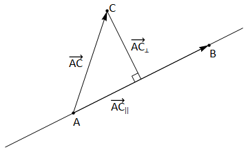
Fig. 3.9 The shortest distance from a point \(C\) to a line is given by \(d=|\overrightarrow{AC}_{\perp}|\).

This distance is equal to the height of the parallelogram spanned by vectors \(\overrightarrow{AB}\) and \(\overrightarrow{AC}\), so it can be found using the vector product:

\[d=\frac{|\overrightarrow{AB}\times\overrightarrow{AC}|}{|\overrightarrow{AB}|}\]

Alternatively, we could use the scalar product, since

\[\overrightarrow{AC}=\overrightarrow{AC}_{\parallel}+\overrightarrow{AC}_{\perp}\]

in which the parallel component \(\overrightarrow{AC}_{\parallel}\) is simply the projection of \(\overrightarrow{AC}\) onto \(\overrightarrow{AB}\).

An example would be to find the shortest distance between the point \(C:(5,0,5)\) and the line that passes through the points \(A:(1,1,3)\) and \(B:(3,4,2)\). By using the vector product:

\[\begin{split}\overrightarrow{AB}\times\overrightarrow{AC} &= \begin{vmatrix}\hat{\bf x} & \hat{\bf y} & \hat{\bf z}\\2&3&-1\\4&-1&2\end{vmatrix} = 5\hat{\bf x} - 8\hat{\bf y} - 14\hat{\bf z} \\ d &= \frac{|\overrightarrow{AB}\times\overrightarrow{AC}|}{\overrightarrow{AB}}=\sqrt{\frac{285}{14}}\end{split}\]

Or by using the scalar product:

\[\begin{split}\overrightarrow{AB} &= \begin{pmatrix}2\\3\\-1\end{pmatrix}\\ \overrightarrow{AC} &= \begin{pmatrix}4\\-1\\-2\end{pmatrix} \\ |\overrightarrow{AC}_{\parallel}| &= \overrightarrow{AC}.\frac{\overrightarrow{AB}}{|\overrightarrow{AB}|}=\frac{3}{\sqrt{14}} d &= \sqrt{|\overrightarrow{AC}|^2-|\overrightarrow{AC}_{\parallel}|^2}=\sqrt{21-\frac{3}{14}}=\sqrt{\frac{285}{14}}\end{split}\]

3.7.4. Shortest Distance to a Plane

The shortest distance between a point \(P\) and a plane containing the point \(A\) is the perpendicular distance, marked \(d\) in Fig. 3.10

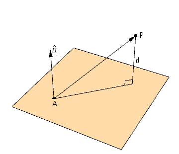
Fig. 3.10 The shortest distance from a point \(P\) to a plane through \(A\) is the projection of \(\overrightarrow{AP}\) onto the unit normal

This distance is the given by projecting vector \(\overrightarrow{AP}\) onto the unit normal:

\[d=|\overrightarrow{AP}.\hat{{\bf n}}|\]

The shortest distance between a line and a (non-intersecting) plane, two parallel planes, or two skew lines can be found in the same way, by picking any point on each line/plane. The case of two skew lines is illustrated in Fig. 3.11

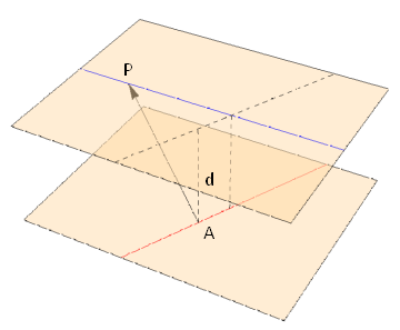
Fig. 3.11 The shortest distance between two skew lines illustrated.

An example here would be to find the shortest distance between the planes:

\[\begin{split}P_1:&&\, 3x-2y+4z=12 \\ P_2:&&\, 6x-4y+8z=8\end{split}\]

Given that the two planes are parallel, with normal direction

\[\begin{split}{\bf n}=\left(\begin{array}{c}3\\-2\\4\end{array}\right)\end{split}\]

We have to pick a point on each plane - For example, on \(P_1\) lets pick the point \(A:(0,0,3)\) and on \(P_2\) lets pick the point \(B:(0,0,1)\). The distance between the two planes is therefore given by:

\[|\overrightarrow{AB}.\hat{{\bf n}}|=\frac{|(0,0,-2).(3,2,-4)|}{\sqrt{3^2+2^2+4^2}}=\frac{8}{\sqrt{29}}\]

previous

2. Integration Preliminaries

next

4. Vector Fields